What is R?

R is an open source programming language well suited for data analysis and visualization [@r]. It is a powerful language used in mathematical operations, data-processing, analysis and graphical display of data. Like other statistical software, R provides a statistical framework and terminal–based interface for users to parse commands for data ingestion, manipulation and graphics. @xia pointed out that R is a vehicle for newly developing methods of interactive data analysis. R have rapidly developed and extended its capability to a large collection of packages provided by researchers and volunteers. R can be downloaded from https://www.r-project.org and available for all thre major operating systems—Windows, Mac and Unix/Linux.

R is an interpreted language—the expression specified in this languages executes line by line similar to other languages like python or ruby rather than compiling the source code an executable chunk as in C++. One of the power of R language is its dynamic—infers the data types of the variables based on the context. We do not need to declare variables separately. R is considered as esoteric because its syntax are easily understood by people from different fields.

The R programming usage has become one-stop solution to data analysis. R was created in 1993 and has evolved into a stable programming language. It has become a de facto standard for data analysis both in academic and industry sectors. R has its roots in the statistics community, being created by statistians for statistics. Many of its core tools are directed toward statistics. Being an open-source language, R has many advantage oover other commercial statistical platform like MATLAB, SAS and SPSS. The big rip for using R is its ecosystem of packages.

Installing R

There is an active community of R developers which regularly releases a new version R. Each version has a name assigned to it. Except for major resease, the version of R are usually backward compatible in terms of their funcitonality. Installing R is fairly straightforward. R is available on most computing platform like Windows. Linux and Mac. It is highly recommended to install a pre–compiled bindary distribution for your operating system. Follow this instructions to install R

• Go to https://cran.r-project.org/
• Click download latest version of R for Mac or Windows. For Windows users click Base and download the installer. For Mac users select the file R-3.x.x.pkg that aligns with yur OS version.
• After you download the installer, double-click its icon and the compiled binary executes and install R in your machine. Follow the instruction to install R in default location.

Once you have installed R, you should now have an icon on your Windows or Mac desktop labelled R. If you are using Ubuntu, in the Applications menu, you should see a new group named Programming with the application R. After the installation of R, the software is launched by Double-click the icon and you should see a window that look similar to figure 1 popup. The default desktop layout include the console, which provide the interface between the software and the user, i.e., it accepts R commands typed after the prompt sign >.

Figure 1: The graphical user interface of R

Let’s enter some commands at the prompt, beggining with the following:

print("Programming is fun!, sometimes challenging and occasionnaly frustrating"). Make sure the text you typed inside the print() are either double or single quoted. Press Enter on your keyboard when you’ve finished typing the line.

print("Programming is fun!, sometimes challenging and occasionnaly frustrating")

[1] "Programming is fun!, sometimes challenging and occasionnaly frustrating"

If you have entered the text correctly, the word should appear in the console and the prompt should reappear to let you know that the console is ready to accept more commands.

The version and common packages used in this book can be accessed by simply passing a commands devtools::session_info() in the console. you can also check the version of R installed in your computer with the base version() function

version

               _                           
platform       x86_64-w64-mingw32          
arch           x86_64                      
os             mingw32                     
system         x86_64, mingw32             
status                                     
major          4                           
minor          0.3                         
year           2020                        
month          10                          
day            10                          
svn rev        79318                       
language       R                           
version.string R version 4.0.3 (2020-10-10)
nickname       Bunny-Wunnies Freak Out     

By default, R stores all of your R–related files in the startup folder named R. You can check the path of the current working directory with the getwd() function.

getwd()

[1] "D:/semba/myblog/content/post/2020-01-01-basics-of-r-programming"

Alternatively, you can create a personal working directory in which to read your files into R and also to export the files generated from processes in R. You should then define the path of the working directory using the setwd() function.

setwd("E:/bookdown/spatil_r/")

To see which files are in the working directory that you just defined or the default R working directory use the list.files() function

list.files()

What is RStudio?

You have seen that R comes with a console that allows to program interactively. However, you need to install RStudio— an integrated development environment (IDE) for R programming. RStudio makes writing R codes easier and in a more user-friendly environment [@xia]. RStudio is a free and open-source integrated development environment (IDE) for R [@rstudio]. You must have already installed R in your machine before you install Rstudio. You can download the software from the R-studio website at this link http:/www.rstudio.com.

Rstudio work in the four operating systems—Windows, Mac, Ubuntu and Fedora. To obtain the reference infomation for citing RStudio in publication by simply typing RStudio.version() command in the console.

Basic Features of RStudio

After the installation is complete, open Rstudio and a window like the one shown in figure (Figure 2 should open. Across the top is a standard menu bar with typicall menu items. Below the standard menu, the program is divided into different panels. The four fundamental panels in Rstudio that we will look are editor, console, worksapce and plots.

Figure 2: The graphical user interface of RStudio showing the four main windows

• source editor and data viewer: The top left corner contains the script editor. This a simple text editor for writing and editing R scripts and markdown documents. Several tabs can be opened in the editor window at once, with each tab representing a different document. These files can be saved from the editor into the working directory. The editor window is also used to view data frame similar to Excel spreadsheet. Source editor is recommended in most programming work because of its efficient way to manage scripts and Rmarkdown document for reproducible work.

• environment (workspace): The top right panel contains several tabs but I introduce the workspace and history tabs. The workspace list all the objects that are currently loaded in R’s memory. You can use the ls() function to check the list all files in the environment.You can also view the object in the workspace (environment) by clicking them or run View() function in console.

• history tab provides a record of the recent commands executed in the console, scripts or rmarkdown documents.

• R consoles: The bottom left window is the command line widely known as console. this window is similar to console in base R. This is used to directly enter commands into R. There are only few thing you need to know to become familiar with console. Click in the console and you should see a blicking caretappear next to the greater than sign >, reffered as prompt. This is where you will type R’comands to executes one command at a time. For example, in a console type the 2+3 and click enter;

7+8

[1] 15

Once you have entered commands here, press enter to execute the command and you will get the answer 25. The console is useful for entering single lines of code and running them. Oftentime this occurs when you are exploring or testing a certain task with a combinations of functions and objects. But because coding is all about creating scripts that automate the analytical process, you will find that very rare you use the the console but rather write the code in script or markdown files.

• files, plots, packages, help, and viewer: The bottom-right window has five tabs for files, plots, package, help and viewer. The files tab allows browsing of the computers file directory. The plots tab will show recent plots and figures drawn with graphic functions in R. The packages tabl list all packages installed in R and provide tools for download new package and update packages. The help tab is an invaluable tab, it help to search for functions and see examples of how they are used. The viewer tab is like the plot tab that both are used to show recent plots and figures. However, while the plots is for static plot, the viewer is for animations and interactive plots and figures.

An important concept in R is the current working directory. This is the file folder that R points to by default. By default the software stores all of your R-related files in the startup folder, which is the Document folder. Alternatively, you can create a personal working directory in which to store your R-related files with the setwd() function. This is especially important when reading in data to R. The current working directory should be set to the folder containing the data to be loaded into R.

Rstudio editor

You should be making use of Rstudio’s text edditor to code in R. It is important to practice writing good code that are easy to read and understand what they mean. In short make sure your code is easy to read and understand what it does. This will help you understand your own code later, and help other people understand your code when shared or when they ask you for a help.

Rmarkdown

Rstudio’s text editor allows to create markdown files called rmarkdown. Markdown is a plain text that combine codes and text and ability to ouput different format like word, PDF and HTML format. This ability of combining text and code has made rmarkdown a powerful markup language in R. In general, with rmarkdown you can write document with titles, headings, paragraphs, insert figures, tables and equations.

Another useful feature of rmarkdown document is the option to publish R projects in various file format such as HTML, Latex, PDF EPUB, Word and many others. This feature enables you to share your results with colleagues who may or may not have R software. The published document includes formated plain text in section, heading and paragraphs that comes with code chunk, figures and tables.

Use descriptive names

While programming, you will often declare and assign names of the variables. R usually will not care what name you give to any variables. But declare a descriptive name is informative because you easily remember what it contains. Therefore, its is encouraged to give names that represent the meaning of the data stored in each variable.

Use comments

While working with R script, the hash tag # set a comment and tell the script to skip the line with the hash tag. In rmarkdown, the hash tag are used to set headings and therefore you can specify the comment with hash tage in the chunk code. Comments are useful as they help you and other people about a particular code and what particular aspect it does. Therefore, it is always recommend to write clear and precise comments that can help you in the future when you want to understand what the code does and also can help others follows with little consultation if shared.

Getting Help in R

Often, we get stuck whilee doing some analysis as either we do not know the correct function to use or its syntax. Its important for anyone who is new to R to knwo the right place to look for help. There are two ways to get help in R—built in help system and online.

?help.start()

help("metR::Adiabat")
?metR::Adiabat

help.search("geom_contour")
??ggplot2::geom_abline

demo()

example("t.test")

t.test> require(graphics)

t.test> t.test(1:10, y = c(7:20))      # P = .00001855

    Welch Two Sample t-test

data:  1:10 and c(7:20)
t = -5.4349, df = 21.982, p-value = 1.855e-05
alternative hypothesis: true difference in means is not equal to 0
95 percent confidence interval:
 -11.052802  -4.947198
sample estimates:
mean of x mean of y 
      5.5      13.5 


t.test> t.test(1:10, y = c(7:20, 200)) # P = .1245    -- NOT significant anymore

    Welch Two Sample t-test

data:  1:10 and c(7:20, 200)
t = -1.6329, df = 14.165, p-value = 0.1245
alternative hypothesis: true difference in means is not equal to 0
95 percent confidence interval:
 -47.242900   6.376233
sample estimates:
mean of x mean of y 
  5.50000  25.93333 


t.test> ## Classical example: Student's sleep data
t.test> plot(extra ~ group, data = sleep)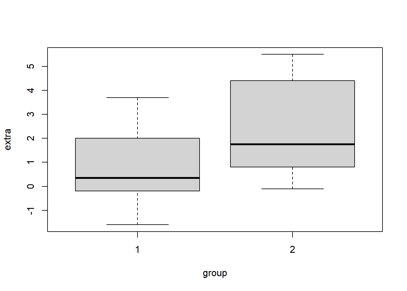

t.test> ## Traditional interface
t.test> with(sleep, t.test(extra[group == 1], extra[group == 2]))

    Welch Two Sample t-test

data:  extra[group == 1] and extra[group == 2]
t = -1.8608, df = 17.776, p-value = 0.07939
alternative hypothesis: true difference in means is not equal to 0
95 percent confidence interval:
 -3.3654832  0.2054832
sample estimates:
mean of x mean of y 
     0.75      2.33 


t.test> ## Formula interface
t.test> t.test(extra ~ group, data = sleep)

    Welch Two Sample t-test

data:  extra by group
t = -1.8608, df = 17.776, p-value = 0.07939
alternative hypothesis: true difference in means is not equal to 0
95 percent confidence interval:
 -3.3654832  0.2054832
sample estimates:
mean in group 1 mean in group 2 
           0.75            2.33 


t.test> ## Formula interface to one-sample test
t.test> t.test(extra ~ 1, data = sleep)

    One Sample t-test

data:  extra
t = 3.413, df = 19, p-value = 0.002918
alternative hypothesis: true mean is not equal to 0
95 percent confidence interval:
 0.5955845 2.4844155
sample estimates:
mean of x 
     1.54 


t.test> ## Formula interface to paired test
t.test> ## The sleep data are actually paired, so could have been in wide format:
t.test> sleep2 <- reshape(sleep, direction = "wide", 
t.test+                   idvar = "ID", timevar = "group")

t.test> t.test(Pair(extra.1, extra.2) ~ 1, data = sleep2)

    Paired t-test

data:  Pair(extra.1, extra.2)
t = -4.0621, df = 9, p-value = 0.002833
alternative hypothesis: true difference in means is not equal to 0
95 percent confidence interval:
 -2.4598858 -0.7001142
sample estimates:
mean of the differences 
                  -1.58 

library(help = "metR")

?vignette()

vignette(all = FALSE)

vignette( package = "sf")