
Begginer guide: get familar with coding in R
In the previous post, you installed and got a glimpse of R and Rstudio program. In this chapter you begin to do something with them. We will begin with some simple calculations and then move on to variables. We then move to functions and later to packages. We will learn the basic data types that are widely used in R and how to construct them
This chapter provides example of foundational programming concepts in R. These include the basic tasks like importing data in R, manipulating data, visualizing the data and conduct explatory and inferencial statistics. These basics will provide building blocks for handling data, analysing data and make plots with R. In the examples, R codes are presented in the light gray chunk blocks. Inside these chunk blocks, lines that begin with two number signs (##) are the outputs of the preceding lines of codes that have been executed and lines without the number signs are are the code that generated the output.
Maths in R
Before proceeding, we need to clear the workspace by typing;
rm(list = ls())Clearing the workspace before you begin a new project is an important task in R because it avoid name conflicts with previous projects. We can also clear figures from the plot windows by simply typing;
graphics.off()Creating a vector files of numerical number of strings in R is easy. To combine more than one element in a vector simply use the c function, which stands for concatenate.
age = c(45,75,65,85,45,32,57,65,52,45,65,32,89,45,66)which first assign age as the name of the object, then combine the list of elements in paretheses with c function.
R operators
R provides standard arithmetic operators for addition , substraction, multiplication, division, and exponential. The basic symbols used by R to perform mathematical operations are called operators. Some of the mathematical operators are listed in table 1. Note that the forward slash (/) is used for division because it’s similar to the division line that you would use when writing a fraction.
require(magrittr)

data.frame(Symbol = c("+", "-", "*", "/"),
           Operation = c("Addition", "Substraction","Multiplication","Division")) %>%
knitr::kable(format = "html", align = "l", caption = "Basic R operators")| Symbol | Operation |
|---|---|
|
|
Addition |
|
|
Substraction |
|
|
Multiplication |
| / | Division |
Because of the convinient, we will use Rstudio console, just write an expression 2 + 3 and click Enter
2+3[1] 5As we expected, R returns the answer as 5. Unlike other programming languages, coding in R does not need to terminate the expression or lines with a semicolon.
10-4[1] 623*2[1] 468/2[1] 45^2[1] 255%%3[1] 25%%5[1] 0Precedence
R can be used to express complicated mathematical formulas. For anyone unfamiliar with writing formulas on computers, it is important to recognize that R will make assumptions about which part of the formulas to compute first. This order of operations is referred as predecence. Multiplication and division have a higher order than addition and subtraction. For example guess what is the answer for the mathematical expression in the chunk below.
5 - 3 + 8 / 2 * 3The answer should be 14. According precedence, the number 8 is first divided by 2 to get 4 as product which is multiplied by 3 to obtain 12 and then 5 is added to get 17, which is substracted by 3 to get 14 as final result. We use parentheses in a R to control the order of operations like in the expression below. Can you make a mental calculation and provide the answer before you click enter for the expression in the chunk below?
5 - (3 + 8) / 2 * 3The result of the expression is -11.5 and not 14 because the parentheses tell R to do the operation in the parentheses firs and then do the operation outside the parentheses.
Assignment operator
We often use an assignment operator to assing the value of an expression to a variable. R has two assignment operators—the conventional assignment operator =, which is present in most programming languages, and the arrows <- and -> which are specific to R. The expression x = 5 assign the value 5 to x, likewise the expression x <- 5 and 5 -> x have the same effect. Throughout this book, we stick on the conventional assignment operator (=)
Variables
We can create expression using variables. for instance, we assign the value 5 to the variable x and evaluate the square of x using the exponential ^ operator.
x = 5
x^2
[1] 25R has many types of variables that store different kinds of data in different ways. Example you can store a list of numbers or text
days= c("Monday", "Tuesday", "Wednesday")
speed  = c(128, 158, 89)
R has peculiar syntax when it comes to variable names. The dot character . has a completely different meaning as compared to other programming languages. In R, we can use . in the variable names, so x.1 and x_1 are perfectly valid. In practice, the dot operator is used as a visual separator in variable names, similar to underscore in most other programming languages.
Naming conventions
- Name must begin with a letter. Do not use number, dollar sign or underscore
- R is case sensitive; average and Average are two different objects in R
- Use descriptive names
- if the name is made of more than one word, used period (. or underscore to separate the words)
Functions
Functions in R are first class objects, which means that they can be treated much like any other R object. Importantly,
- Functions can be passed as arguments to other functions
- Functions can be nested, so that you can define a function inside of another function
The return value of a function is the last expression in the function body to be evaluated.
R functions arguments can be matched positionally or by name. So the following calls to sd are all equivalent
data = rnorm(25)
sum(data)
[1] 2.875542sd(data)[1] 0.9071268mean(data)[1] 0.1150217median(data)[1] 0.1755854Essential functions
R has many built-in functions that can be used fo a great variety of tasks. These can be suplemented with packages, which contains more functions bundled in one document. Here is a list of common and widely used functions
+ rep() — repeates a value some number of times to make a list
+ seq() — creates a sequence of values between a start and end number and spaced at certain interval
+ aggregate() — used to bin data by condition
+ table() — used to summarise categorical data
+ plot() — graphical plots of data
+ hist() — a function for plotting a histogram
+ boxplot() — a function for plotting boxplot
+ mean() — compute arithmetric mean
+ sd() — compute arithmetric standard deviation
+ sum() — compute the total of the set of elements
+ length() — function to count the number of elements in a vector
Setting Working Directory
@xia defined a working directory as a folder in your computer or server where you stores the raw data, codes and output for that specific project. This folder is important in programming because it allows to read the data and write outputs to this working directory. In R you can set working directory with setwd() function and check whether you are in the right working directory with the getwd() function.
getwd()

setwd("./Data Manipulation/R_dege/")
Packages or Libraries
R is made up of many user-written package. The base version of R allows user to get started in R, but the capabilities of base R are limited and additional packages are required for smooth performance of working with data. packages are collections of R functions, data, and compiled code in a well-defined format. A package bundles together code, data, documentation and tests and provide ana easy method to share with others. Until November 2018, there were 1300+ packages available for download on CRAN and countless more avaialble trought GitHub. The huge number of package has made R so successful and the chance is that some one has already created a package that can solve the problem you about to tackle and you can benefit from their work by downloading their package.
Installing packages
R comes with a standard set of packages. Others are available for download and installation. The primary of stable package is the CRAN. In R you can install a package from CRAN with an install.packages("packagename") function that allows you to install the package you want to use into R. In have already installed the ggplot2 packages in my machine, so if you want to install in your machine you can simply uncomment the chunk below by removing the hash tag (#)
## install.packages("ggplot2")
## install.packages("dplyr")
## install.packages("lubridate")
## install.packages("factoextra")
## install.packages("readxl")
## install.packages("kableextra")
## install.packages("haven")
## install.packages("readr")
Loading packages
Once package is downloaded and installed in your computer, you have to them into the session to access its functions and resources of the package. Yu can load the packages you want ot use with ether library() or required() function.
require(dplyr)
library(readr)
require(lubridate)
library(readxl)
require(haven)
library(ggplot2)
require(kableExtra)
Understanding Data in R
Clearing the workspace is always recommended before working on a new R project to avoid name conflicts with provious projects. We can also clear all figures using graphics.off()' function and clear the console with a combinantion ofCTRL+L`. It is a good code practise that a new R project start with the code in the chunk below:
rm(list = ls())
graphics.off()
Data Types
R is a flexible language that allows to work with different kind of data format [@bradley]. This inluced integer, numeric, character, complex, dates and logical. The default data type or class in R is double precision—numeric. In a nutshell, R treats all kind of data into five categories but we deal with only four in this book. Before proceeding, we need to clear the workspace by typing rm(list = ls()) after the prompt in the in a console.
Integers:Integer values do not have decimal places. They are commonly used for counting or indexing.
aa = c(20,68,78,50)You can check if the data is integer with is.integer() and can convert numeric value to an integer with as.integer()
is.integer(aa)[1] FALSEYou can query the class of the object with the class() to know the class of the object
class(aa)[1] "numeric"Although the object bb is integer as confirmed with as.integer() function, the class() ouput the answer as numeric. This is because the defaul type of number in r is numeric. However, you can use the function as.integer() to convert numeric value to integer
class(as.integer(aa))[1] "integer"Numeric: The numeric class holds the set of real numbers — decimal place numbers. The numeric class is more general than the integer class, and inclused the integer numbers.
These could be any number (whole or decimal number). You can check if the data is integer with is.integer()
bb = c(12.5, 45.68, 2.65)
class(bb)
[1] "numeric"is.numeric(bb)[1] TRUEStrings: These collection of characters. This often aretextdata like names. You can check if the data is integer withis.character()
kata = c("Dege", "Mchikichini", "Mwembe Mdogo", "Cheka")
class(kata)
[1] "character"Factor: These are strings from finite set of values. For example, we might wish to store a variable that records gender of people. You can check if the data is factor withis.factor()and useas.factor()to convertstringtofactor
sex = c("Male", "Female", "Male", "Male", "Female")
sex = as.factor(sex)
class(sex)
[1] "factor"levels(sex)[1] "Female" "Male" Often times we need to know the possible groups that are in the factor data. This can be achieved with the levels() function
levels(sex)[1] "Female" "Male" levels(kata)NULLOften we wish to take a continuous numerical vector and transform it into a factor. The function cut() takes a vector of numerical data and creates a factor based on your give cut-points. Let us make a fictional income of 508 people with rnorm() function.
income = rnorm(n = 508, mean = 500, sd = 80)
hist(income, col = "green", main = "", las = 1, xlab = "Individual Income")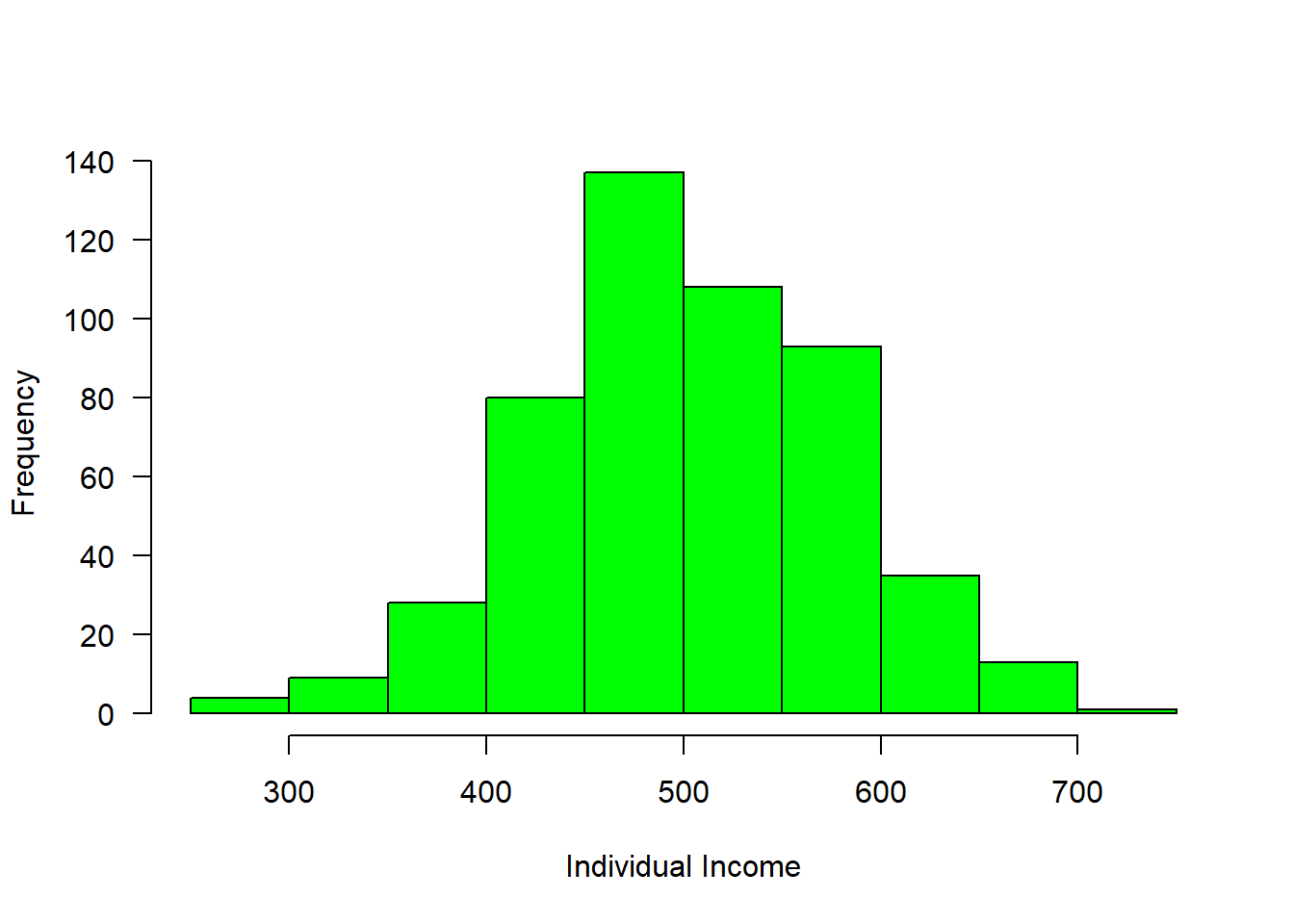
Figure 1: Income distribution
#mosaic::plotDist(dist = "norm", mean = 500, sd = 80)We can now breaks the distribution into groups and make a simple plot as shown in figure 2, where those with income less than 400 were about 50, followed with a group with income range between 400 and 500 of about 200 and 250 people receive income above 500
group = cut(income, breaks = c(300,400,500,800),
            labels = c("Below 400", "400-500", "Above 500"))
is.factor(group)
[1] TRUElevels(group)[1] "Below 400" "400-500" "Above 500"barplot(table(group), las = 1, horiz = FALSE, col = c("blue", "red", "blue"), ylab = "Frequency", xlab = "Group of Income")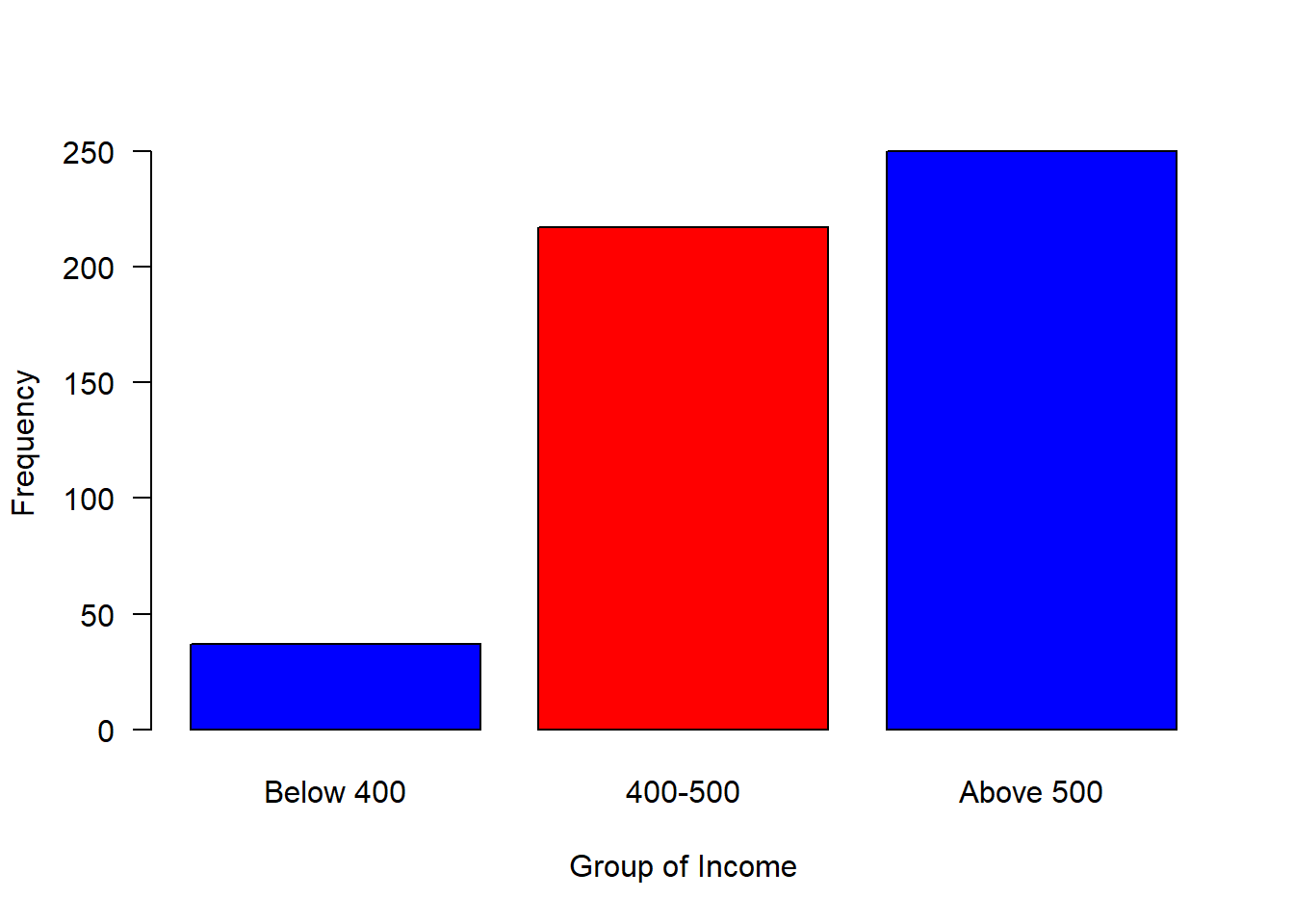
Figure 2: Barplot of grouped income
data = data.frame(group, income)Logicals: This is a special case of a factor that can only take on the valuesTRUEandFALSE. R is case-sensitive, therefore you must always capitalizeTRUEandFALSEin function in R.Date and time
Vectors
Ofen times we want to store a set of numbers in once place. One way to do this is using the vectors in R. Vectors store severl numbers– a set of numbers in one container. let us look on the example below
id = c(1,2,3,4,5)
people = c(158,659,782,659,759)
street = c("Dege", "Mchikichini", "Mwembe Mdogo", "Mwongozo",  "Cheka")
Notice that the c() function, which is short for concatenate wraps the list of numbers. The c() function combines all numbers together into one container. Notice also that all the individual numbers are separated with a comma. The comma is reffered to an an item-delimiter. It allows R to hold each of the numbers separately. This is vital as without the item-delimiter, R will treat a vector as one big, unsperated number.
Indexing the element
One advantage of vector is that you can extract individual element in the vector object by indexing, which is accomplished using the square bracket as illustrated below.
id[5][1] 5people[5][1] 759street[5][1] "Cheka"Apart from extracting single element, indexing allows to extract a range of element in a vector. This is extremely important because it allows to subset a portion of data in a vector. A colon operator is used to extract a range of data
street[2:4][1] "Mchikichini" "Mwembe Mdogo" "Mwongozo" Adding and Replacing an element in a vector
It is possible to add element of an axisting vecor. Here ia an example
id[6] = 6
people[6] = 578
street[6] = "Mwongozo"
Sometimes you may need to replace an element from a vector, this can be achieved with indexing
people[1] = 750Number of elements in a vector
Sometimes you may have a long vector and want to know the numbers of elements in the object. R has length() function that allows you to query the vector and print the answer
length(people)[1] 6Data Frame
data.frame is very much like a simple Excel spreadsheet where each column represents a variable type and each row represent observations. Perhaps the easiest way to create a data frame is to parse vectors in data.frame() function.
# create vectors
Name  = c('Bob','Jeff','Mary')
Score = c(90, 75, 92)

dt = data.frame(Name, Score)
Table 2 show the the data frame created by fusing the two vectors together.
| Name | Score |
|---|---|
| Bob | 90 |
| Jeff | 75 |
| Mary | 92 |
Because the columns have meaning and we have given them column names, it is desirable to want to access an element by the name of the column as opposed to the column number.In large Excel spreadsheets I often get annoyed trying to remember which column something was. The $sign and []are used in R to select variable from the data frame.
dt$Name[1] "Bob" "Jeff" "Mary"dt[,1][1] "Bob" "Jeff" "Mary"dt$Score[1] 90 75 92dt[,2][1] 90 75 92R has build in dataset that we can use for illustration. For example, @longley created a longley dataset, which is data frame with 7 economic variables observed every year from 1947 ti 1962 (Table 3). We can add the data in the workspace with data() function
data(longley)

longley %>%
  kable(caption = "Longleys' Economic dataset", align = "c", row.names = F) %>%
column_spec(1:7, width = "3cm")| GNP.deflator | GNP | Unemployed | Armed.Forces | Population | Year | Employed |
|---|---|---|---|---|---|---|
| 83.0 | 234.289 | 235.6 | 159.0 | 107.608 | 1947 | 60.323 |
| 88.5 | 259.426 | 232.5 | 145.6 | 108.632 | 1948 | 61.122 |
| 88.2 | 258.054 | 368.2 | 161.6 | 109.773 | 1949 | 60.171 |
| 89.5 | 284.599 | 335.1 | 165.0 | 110.929 | 1950 | 61.187 |
| 96.2 | 328.975 | 209.9 | 309.9 | 112.075 | 1951 | 63.221 |
| 98.1 | 346.999 | 193.2 | 359.4 | 113.270 | 1952 | 63.639 |
| 99.0 | 365.385 | 187.0 | 354.7 | 115.094 | 1953 | 64.989 |
| 100.0 | 363.112 | 357.8 | 335.0 | 116.219 | 1954 | 63.761 |
| 101.2 | 397.469 | 290.4 | 304.8 | 117.388 | 1955 | 66.019 |
| 104.6 | 419.180 | 282.2 | 285.7 | 118.734 | 1956 | 67.857 |
| 108.4 | 442.769 | 293.6 | 279.8 | 120.445 | 1957 | 68.169 |
| 110.8 | 444.546 | 468.1 | 263.7 | 121.950 | 1958 | 66.513 |
| 112.6 | 482.704 | 381.3 | 255.2 | 123.366 | 1959 | 68.655 |
| 114.2 | 502.601 | 393.1 | 251.4 | 125.368 | 1960 | 69.564 |
| 115.7 | 518.173 | 480.6 | 257.2 | 127.852 | 1961 | 69.331 |
| 116.9 | 554.894 | 400.7 | 282.7 | 130.081 | 1962 | 70.551 |
Sometimes you may need to create set of values and store them in vectors, then combine the vectors into a data frame. Let us see how this can be done. First create three vectors. One contains id for ten individuals, the second vector hold the time each individual signed in the attendane book and the third vector is the distance of each individual from office. We can concatenate the set of values to make vectors.
id  = c(1,2,3,4,5,6,7,8,9,10)

time = lubridate::ymd_hms(c("2018-11-20 06:35:25 EAT", "2018-11-20 06:52:05 EAT",
                 "2018-11-20 07:08:45 EAT", "2018-11-20 07:25:25 EAT",
                 "2018-11-20 07:42:05 EAT", "2018-11-20 07:58:45 EAT",
                 "2018-11-20 08:15:25 EAT", "2018-11-20 08:32:05 EAT",
                 "2018-11-20 08:48:45 EAT", "2018-11-20 09:05:25 EAT"), tz = "")

distance = c(20, 85, 45, 69, 42,  52, 6, 45, 36, 7)
Once we have the vectors that have the same length dimension, we can use the function data.frame() to combine the the three vectors into one data frame shown in table 4
arrival = data.frame(id, time, distance)| IDs | Time | Distance |
|---|---|---|
| 1 | 2018-11-20 06:35:25 | 20 |
| 2 | 2018-11-20 06:52:05 | 85 |
| 3 | 2018-11-20 07:08:45 | 45 |
| 4 | 2018-11-20 07:25:25 | 69 |
| 5 | 2018-11-20 07:42:05 | 42 |
| 6 | 2018-11-20 07:58:45 | 52 |
| 7 | 2018-11-20 08:15:25 | 6 |
| 8 | 2018-11-20 08:32:05 | 45 |
| 9 | 2018-11-20 08:48:45 | 36 |
| 10 | 2018-11-20 09:05:25 | 7 |
tibbles
A tibble is a modern data.frame, which keep keep what has proven to be effective and throw out what is not. Tibbles are data.frames that are llazy and surly—they do not change variable names or types and never do partial matching. Tibbles have an enhanced print_method, which makes them easier to use with large dataset containing diffeent objects with large number of variables.
A tibble is created with tibble() function from tibble package [@tibble]
data.tb = tibble::tibble(time, distance)
tibble::is_tibble(data.tb);class(data.tb)
[1] TRUE[1] "tbl_df" "tbl" "data.frame"You can also use the as_tibble() to convert data.frame to tibble
## create a data.frame
data.df = data.frame(time, distance)
## create a tibble
data.tbl = tibble::as_tibble(data.df)
## printout
tibble::is_tibble(data.df); tibble::is_tibble(data.tb)
[1] FALSE[1] TRUEColumn Names
Unlike data.frame that is strict on column names, tibble need not be valid R variable names. They can contain unusual characters like a space or a smiley but be enclosed in ticks.
tibble::tibble(id = 1:10,
               ":" = rep(c("NE", "SE"), each = 5),
               "-" = rnorm(10, 25,2),
               chl = rnorm(10,.25,.01))
# A tibble: 10 x 4
id `:` `-` chl
<int> <chr> <dbl> <dbl>
1 1 NE 22.4 0.246
2 2 NE 24.4 0.250
3 3 NE 22.2 0.258
4 4 NE 24.8 0.263
5 5 NE 22.1 0.239
6 6 SE 28.4 0.247
7 7 SE 21.2 0.253
8 8 SE 26.4 0.246
9 9 SE 26.5 0.255
10 10 SE 27.4 0.242However, when we use data.frame()instead of tibble() with the same arguments, we notice that the data.frame() function has modified the column names.
data.frame(id = 1:10,
           ":" = rep(c("NE", "SE"), each = 5),
           "-" = rnorm(10, 25,2),
           chl = rnorm(10,.25,.01))
id X. X..1 chl
1 1 NE 23.54136 0.2392456
2 2 NE 26.30564 0.2516395
3 3 NE 28.08723 0.2420568
4 4 NE 26.36949 0.2482949
5 5 NE 23.30528 0.2553076
6 6 SE 27.58529 0.2332887
7 7 SE 25.80831 0.2552407
8 8 SE 22.65104 0.2502862
9 9 SE 25.10100 0.2497607
10 10 SE 24.84666 0.2503427Add rows and columns
tibble allows you to add column and rows. Let us add the unique ID in the data.tb we created earlier using add_column() function. This function allows us to specify wher we want to place the column we will create. for this case we want the id variable to be the first, hence we specify .before = 1 argument.
tibble::add_column(.data = data.tb, id = 1:10, .before = 1)# A tibble: 10 x 3
id time distance
<int> <dttm> <dbl>
1 1 2018-11-20 06:35:25 20
2 2 2018-11-20 06:52:05 85
3 3 2018-11-20 07:08:45 45
4 4 2018-11-20 07:25:25 69
5 5 2018-11-20 07:42:05 42
6 6 2018-11-20 07:58:45 52
7 7 2018-11-20 08:15:25 6
8 8 2018-11-20 08:32:05 45
9 9 2018-11-20 08:48:45 36
10 10 2018-11-20 09:05:25 7We can also add row(s) in tibble with the add_row() function and specify at which row location we want to insert the rows. For instance, in the code below, we command the rows to be inserted from row 5
tibble::add_row(.data = data.tb,
                time = seq(lubridate::dmy(120514),lubridate::dmy(150514), by = "day"),
                distance = rnorm(4, 23,6),
                .before = 5)
# A tibble: 14 x 2
time distance
<dttm> <dbl>
1 2018-11-20 06:35:25 20
2 2018-11-20 06:52:05 85
3 2018-11-20 07:08:45 45
4 2018-11-20 07:25:25 69
5 2014-05-12 00:00:00 22.5
6 2014-05-13 00:00:00 18.4
7 2014-05-14 00:00:00 15.1
8 2014-05-15 00:00:00 16.3
9 2018-11-20 07:42:05 42
10 2018-11-20 07:58:45 52
11 2018-11-20 08:15:25 6
12 2018-11-20 08:32:05 45
13 2018-11-20 08:48:45 36
14 2018-11-20 09:05:25 7 Exercise
- Create a vector of character strings with six elements
test <- c('red','red','blue','yellow','blue','green')and then
- Transform the test vector just you created into a factor.
- Use the
levels()command to determine the levels (and order) of the factor you just created. - Transform the factor you just created into integers. Comment on the relationship between the integers and the order of the levels you found in part (b).
- Use some sort of comparison to create a vector that identifies which factor elements are the red group.
- Suppose we vectors that give a students name, their GPA, and their major. We want to come up with a list of forestry students with a GPA of greater than 3.0.
Name <- c('Adam','Benjamin','Caleb','Daniel','Ephriam', 'Frank','Gideon')
GPA <- c(3.2, 3.8, 2.6, 2.3, 3.4, 3.7, 4.0)
Major <- c('Math','Forestry','Biology','Forestry','Forestry','Math','Forestry')- Create a vector of TRUE/FALSE values that indicate whether the students GPA is greater than 3.0.
- Create a vector of TRUE/FALSE values that indicate whether the students’ major is forestry.
- Create a vector of TRUE/FALSE values that indicates if a student has a GPA greater than 3.0 and is a forestry major.
- Convert the vector of TRUE/FALSE values in part (c) to integer values using the as.numeric() function. Which numeric value corresponds to TRUE?
- Sum (using the sum() function) the vector you created to count the number of students with GPA > 3.0 and are a forestry major.
Exercise
- Create a data.frame named my.trees that has the following columns:
Girth = c(8.3, 8.6, 8.8, 10.5, 10.7, 10.8, 11.0)
Height= c(70, 65, 63, 72, 81, 83, 66)
Volume= c(10.3, 10.3, 10.2, 16.4, 18.8, 19.7, 15.6)- Extract the third observation (i.e. the third row)
- Extract the Girth column referring to it by name (don’t use whatever order you placed the columns in).
- Print out a data frame of all the observations except for the fourth observation. (i.e. Remove the fourth observation/row.)
