Estimate the length at maturity of fish in R

Data

We selected Decapterus kurroides to illustrate ogive graph. These data was collected from the field survey targeting Decapterus kurroides between 2018 and 2020. During the survey scientist selected a random sample of fish and recorded total length (cm), gutted weight (g), gonad weight (g), and maturity stage. Although both sexes were collected in these random samples, we only considered females in this study because the macroscopic staging of testes is difficult to assess. A total of 65 217 gonads were assigned to a macroscopic maturity stage according to the maturity scale of Balbontín and Fischer (1981). This scale defined six stages for Chilean hake: virgin (Stage 1), immature (Stage 2), maturation (Stage 3), maturation with recent spawning (Stage 4), spawning (Stage 5), and spent (Stage 6).

A total of 1214 gonads collected during 2001 were analysed by the means of histology. Gonads were preserved in 10% buffered formalin. The sampling protocol included the dehydration of 3 mm thick subsamples of preserved gonad tissue embedded in paraffin. Sections, 5 μm wide, were stained with Harris’s haematoxylin and eosin was used to analyse and characterise the gonad development and thus determine the different maturity stages according to the modified scale of Herrera et al. (1988): virgin (Stage 1), immature (Stage 2), early maturing (Stage 3), late maturing (Stage 4), mature (Stage 5), ripe (Stage 6), spawning (Stage 7), partial post-spawning (Stage 8), and spent (Stage 9)

require(sizeMat)
require(tidyverse)

deca = read_csv("decapterus_spp.csv")

fm = y ~ poly(x, 3)

deca %>%
  filter(tl_cm > 10 & weigth_g < 120) %>% 
  ggplot(aes(x = tl_cm, y = weigth_g))+
  geom_jitter()+
  geom_smooth(method = "lm", formula = fm)+
  theme(panel.grid = element_line(linetype = "dotted"),
        panel.background = element_rect(fill = NA, colour = "black"),
        axis.text = element_text(size = 11, color = "black"), 
        axis.title = element_text(size = 12, color = "black"))+
  scale_y_continuous(limits =  c(20, NA))+
  labs(x = "Total length (cm)", y = "Weight (gram)")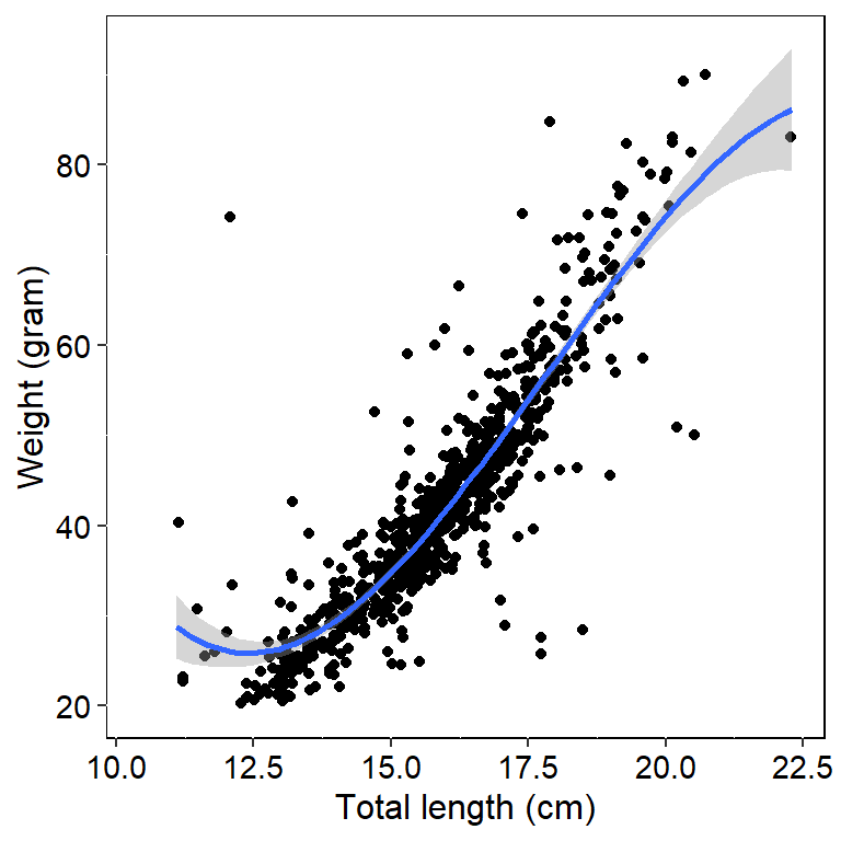

Estimate gonadal maturity

The proportion of mature individuals at age or length, usually called the maturity ogive, is an important population attribute because it directly relates to the reproductive potential of the population. Knowledge of the maturity ogive is especially important in exploited fish populations because it determines the spawning biomass upon which conservation measurements are usually based. The estimation of the maturity ogive commonly consists of three steps.

• First, the spawning season must be identified.
• Second, representative samples of individuals collected during the spawning season are assessed to establish their maturity stage.
• Finally, observed proportions of maturity at length or age are computed which are then conventionally modelled using a logistic function.

The maturity staging process is the most crucial step in estimating the maturity ogive because small errors in stage assignment can lead to profound variations in estimated parameters for the fitted model

deca_mat = sizeMat::gonad_mature(data = deca %>% filter(tl_cm > 10 & weigth_g < 120),
                        varNames = c("tl_cm", "maturity_stage"), 
                        inmName =  c("I","II"), 
                        matName = c("III", "IV", "V"), 
                        method = "fq", 
                        niter = 50)

We print to obtain the statistic of the ogive

deca_mat %>% print()

formula: Y = 1/1+exp-(A + B*X) 

    Original Bootstrap (Median)
A   -20.615  -20.3125          
B   1.5332   1.5022            
L50 13.4461  13.4354           
R2  0.5889   -                 

The statistics can be visualized with an ogive plot

deca_mat %>% plot(onlyOgive = TRUE)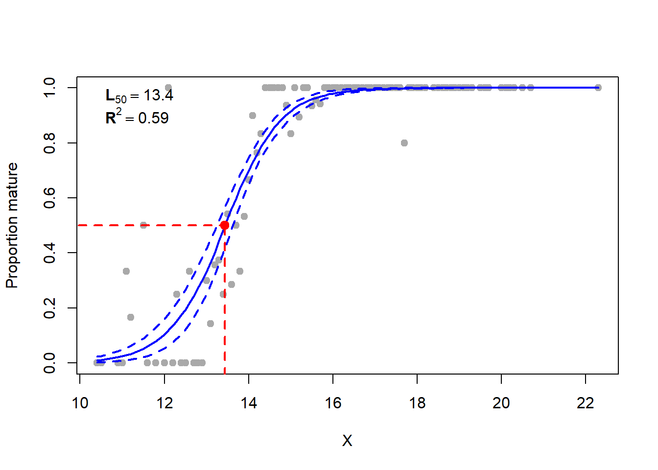

Size at gonad maturity = 13.4 
Confidence intervals = 13.2 - 13.6 
Rsquare = 0.59

df = data.frame(x = 11.2, y = 0.75, label = glue::glue("*r*<sup>2</sup> = {round(0.59, 2)}"))

df.box = data.frame(x = 14, y = 0.55, label = "Age with growth parameters of fishes constitutes essential data to control the dynamic of ichthyologic populations. ")


deca_mat$out %>% as_tibble() %>% 
  ggplot(aes(x = x))+
  geom_line(aes(y = fitted), col = "blue", linetype = "solid", size = 1.2)+
  geom_line(aes(y = CIlower), col = "blue", linetype = 6, size = .8)+
  geom_line(aes(y = CIupper), col = "blue", linetype = 6, size = .8)+
  # modelr::geom_ref_line(h = 0.5, colour = "red", size = 1)+
  theme_bw()+
  theme(panel.grid = element_line(linetype = "dotted"),
        axis.text = element_text(size = 11, color = "black"), 
        axis.title = element_text(size = 12, color = "black"))+
  coord_cartesian(xlim = c(10,18))+
  labs(x = "Total length (cm)", y = "Proportion")+
  geom_segment(aes(x = 10, xend = 13.4461 , y = 0.5, yend = .5), color ="red", size =1.2, linetype = "dashed")+
  geom_segment(aes(x = 13.4461, xend = 13.4461 , y = 0, yend = .5), color ="red", size =1.2, linetype = "dashed") +
  scale_x_continuous(expand = c(0,0), breaks = seq(11,19,2))+
  scale_y_continuous(expand = c(0,0), breaks = seq(0.25,1,.25))+
  geom_text(x = 11.2, y = 0.85, label = expression(L[50]~13.4))+
  ggtext::geom_richtext(data = df, aes(x = x, y = y, label = label))+
  ggtext::geom_textbox(data = df.box, aes(x = x, y = y, label = label),
    width = grid::unit(0.45, "npc"), # 73% of plot panel width
    hjust = 0, vjust = 1)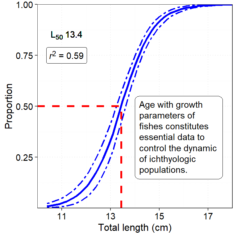

 deca_mat_F = sizeMat::gonad_mature(data = deca %>% filter(tl_cm > 10 & weigth_g < 120 & sex == "F"),
                        varNames = c("tl_cm", "maturity_stage"), 
                        inmName =  c("I","II"), 
                        matName = c("III", "IV", "V"), 
                        method = "fq", 
                        niter = 50)

deca_mat_M = sizeMat::gonad_mature(data = deca %>% filter(tl_cm > 10 & weigth_g < 120 & sex == "M"),
                        varNames = c("tl_cm", "maturity_stage"), 
                        inmName =  c("I","II"), 
                        matName = c("III", "IV", "V"), 
                        method = "fq", 
                        niter = 50)


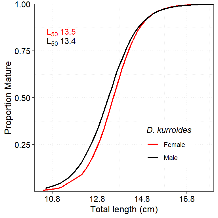
deca_mat_F$out %>% as_tibble() %>% mutate(sex = "Female") %>%
  bind_rows(deca_mat_M$out %>% as_tibble() %>% mutate(sex = "Male")) %>% 
  ggplot(aes(x = x, y = fitted, color = sex))+
  geom_line(size = 0.75)+
  geom_segment(aes(x = 10, xend = 13.5 , y = 0.5, yend = .5), color ="red", size =.25, linetype = "dashed", show.legend = FALSE)+
  geom_segment(aes(x = 13.5, xend = 13.5 , y = 0, yend = .5), color ="red", size =.25, linetype = "dashed", show.legend = FALSE) +
  geom_segment(aes(x = 10, xend = 13.3174 , y = 0.5, yend = .5), color ="black", size =.25, linetype = "dashed", show.legend = FALSE)+
  geom_segment(aes(x = 13.3174, xend = 13.3174 , y = 0, yend = .5), color ="black", size =.25, linetype = "dashed", show.legend = FALSE) +
  scale_x_continuous(expand = c(0,0), breaks = seq(10.8,19,2))+
  scale_y_continuous(expand = c(0,0), breaks = seq(0.25,1,.25))+
  annotate(geom = "text",x = 11.2, y = 0.80, label = expression(L[50]~13.4), color = "black") +
  annotate(geom = "text",x = 11.2, y = 0.85, label = expression(L[50]~13.5), color = "red") +
  theme_bw()+
  theme(panel.grid = element_line(linetype = "dotted"),
        legend.title = element_text(face = "italic"),
        axis.text = element_text(size = 11, color = "black"), 
        axis.title = element_text(size = 12, color = "black"), legend.position = c(.75,.25))+
  coord_cartesian(xlim = c(10,18))+
  scale_color_manual(values = c("red", "black"), name = "D. kurroides")+
  labs(x = "Total length (cm)", y = "Proportion Mature")

cited materials