Familiarize with date and time of Argo Floats data with lubridate package
In this post we will learn to work with date and time data in R. We will use the lubridate package developed by Garrett Grolemund and Hadley Wickham ~@lubridate. This package makes it easy to work with dates and time. Let’s us load the packages that we will use
require(lubridate)
require(tidyverse)
require(magrittr)
require(oce)
Data
We will use the profiles data from Argo within the Indian Ocean. The data was downloaded from the Coriolis Global Data Assembly Center site (ftp://ftp.ifremer.fr/ifremer/argo/) as NetCDF files.
Data processing
The argo profiles were converted from .nc format to data frame. The chunk below briefly describe each step. If you get stuck on the step, consult chapter @ref() that describe looping in details.
There are 52 argo floats measured profiles of temperature and salinity as function of density between 2002-11-11 and 2002-11-11 and made a total of 8419 individual profiles.
Say you want create a column that show the durationof each argo floats in the Indian Ocean. This information is important because it can help identify for on average how long does each float last or identify floats with the shortest or longest operation in the ocean.
To accomplish this task and being able to answer those question, First, the argo floats were aggregated by id. Second, create two variable based on the Id, one variable contain the begin time of the float and the second variable is the end time of the variable. Third, compute the time interval and duration of the float based on the begin and end time. The table 1 show the sample of output resulted from the computation in the chunk below;
floats.duration = argo.ctd.indian %>%
  filter(pressure == 5)  %>%
  group_by(ID) %>%
  summarise(start = first(time),
            end = last(time),
            period = interval(start, end) %>% as.duration() %>% as.numeric("years"),
            count = n()) %>% arrange(count %>% desc())
floats.duration %>%
slice(1,seq(3,52, 6),52) %>%
kableExtra::kable(format = "html", digits = 2, align = "c",
caption = "The period and number of profiles made of randomly selected Argo floats",
col.names = c("Float ID", "Begin", "End", "Duration (years)", "Profile")) %>%
kableExtra::column_spec(column = 1:3, width = "3cm") %>%
kableExtra::column_spec(column = 4, width = "4cm") %>%
kableExtra::add_header_above(c("", "Time of Argo Float" = 2, "", ""))| Float ID | Begin | End | Duration (years) | Profile |
|---|---|---|---|---|
| 5900946 | 2005-05-26 | 2014-12-11 | 9.54 | 333 |
| 1900270 | 2004-11-26 | 2014-01-28 | 9.17 | 320 |
| 1901163 | 2011-05-03 | 2018-06-05 | 7.09 | 259 |
| 1900409 | 2006-10-16 | 2012-11-10 | 6.07 | 219 |
| 1900269 | 2004-11-26 | 2010-02-19 | 5.23 | 181 |
| 1901166 | 2011-05-08 | 2014-12-18 | 3.61 | 131 |
| 1901512 | 2010-10-20 | 2013-11-11 | 3.06 | 105 |
| 1901307 | 2013-06-26 | 2016-02-01 | 2.60 | 95 |
| 1900306 | 2004-01-07 | 2005-12-16 | 1.94 | 66 |
| 1900188 | 2003-09-25 | 2004-10-18 | 1.07 | 38 |
| 2901093 | 2007-12-05 | 2008-01-13 | 0.11 | 5 |
floats.duration %>% filter(period < 2)# A tibble: 8 x 5
ID start end period count
<dbl> <date> <date> <dbl> <int>
1 1900814 2008-11-22 2010-11-12 1.97 68
2 1900306 2004-01-07 2005-12-16 1.94 66
3 1900170 2003-06-27 2005-03-08 1.70 60
4 1900162 2003-06-26 2005-01-13 1.55 54
5 1900186 2003-09-24 2005-03-13 1.47 52
6 2900564 2005-09-16 2006-11-20 1.18 44
7 1900188 2003-09-25 2004-10-18 1.07 38
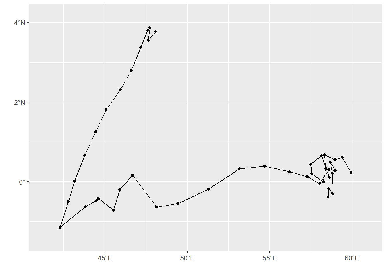
8 2901093 2007-12-05 2008-01-13 0.107 5argo2900564 = argo.ctd.indian %>% filter(ID == 2900564)
ggplot(data = argo2900564 %>% filter(pressure == 5),
aes(x = longitude, y = latitude, group = ID)) + geom_path()+geom_point() +
metR::scale_y_latitude(ticks = 2, expand = c(.1,.1)) +
metR::scale_x_longitude(ticks = 5, expand = c(.1,.1))