
Access Global Climate and Weather Data in R
Climatic change in the last few decades has had a widespread impact on both natural and human systems, observable on all continents. Ecological and environmental models using climatic data often rely on gridded data, such as WorldClim.
WorldClim is a set of global climate layers (gridded climate data in GeoTiff format) that can be used for mapping and spatial modeling. WordlClim version 2 contains average monthly climatic gridded data for the period 1970-2000 with different spatial resolutions, from 30 seconds (~1 km2) to 10 minutes (~340 km2). The dataset includes the main climatic variables (monthly minimum, mean and maximum temperature, precipitation, solar radiation, wind speed and water vapour pressure)
It also provides 19 derived bioclimatic variables (annual mean temperature, mean diurnal range,isothermality, temperature seasonality, max. temperature of warmest month, min. temperature of coldest month, temperature annual range, mean temperature of wettest quarter, mean temperature of driest quarter, mean temperature of warmest quarter, mean temperature of coldest quarter, annual precipitation, precipitation of wettest month, precipitation of driest month, precipitation seasonality (coefficient of variation), precipitation of wettest quarter, precipitation of driest quarter, precipitation of warmest quarter, precipitation of coldest quarter). These layers (grid data) cover the global land areas except Antarctica. They are in the latitude / longitude coordinate reference system (not projected) and the datum is WGS84.
To make it easy to access and download, Robert Hijmans (2017) developed a getData function in raster packaged dedicated to dowload these data directly in R. The aim of this post is to illustrate how we can get these dataset in R and use the power of language to do statistics, modeling and plotting. Before we begin our session, let us first load the packages into our session
Please note that the temperature data are in °C * 10. This means that a value of 231 represents 23.1 °C. This does lead to some confusion, but it allows for much reduced file sizes which is important as for many downloading large files remains difficult. The unit used for the precipitation data is mm (millimeter).
require(tidyverse)
require(sf)
Historical Climate Data
Since we want historical data from worldclim, we must provide arguments var, and a resolution res. Valid variables names are tmin, tmax, prec and bio. Valid resolutions are 0.5, 2.5, 5, and 10 (minutes of a degree). In the case of res=0.5, you must also provide a lon and lat argument for a tile; for the lower resolutions global data will be downloaded. In all cases there are 12 (monthly) files for each variable except for ‘bio’ which contains 19 files.
Maximum temperature
tmax = raster::getData(name = 'worldclim', var = 'tmax', res = 10)We check the class of the dataset with class function
tmax %>% class()[1] "RasterStack"
attr(,"package")
[1] "raster"We get the information that is rasterStack—a collection of raster layer with the same spatial extent and resolution. Let us use dim function to check how many raster layers are there in this rasterstack.
tmax %>% dim()[1] 900 2160 12We see that there are twelve layers—each layer represent a monthly climatological value of maximum temperature from January to December.
tmaxclass : RasterStack
dimensions : 900, 2160, 1944000, 12 (nrow, ncol, ncell, nlayers)
resolution : 0.1666667, 0.1666667 (x, y)
extent : -180, 180, -60, 90 (xmin, xmax, ymin, ymax)
crs : +proj=longlat +datum=WGS84 +no_defs
names : tmax1, tmax2, tmax3, tmax4, tmax5, tmax6, tmax7, tmax8, tmax9, tmax10, tmax11, tmax12
min values : -478, -421, -422, -335, -190, -94, -59, -76, -153, -265, -373, -452
max values : 418, 414, 420, 429, 441, 467, 489, 474, 441, 401, 401, 413 We have noticed that the layer names are not descriptive, we know from our experience that the layers represent months, start from January all the way to December. Therefore, we need to change the layers name to a more descriptive variable names.
names(tmax) = c("Jan", "Feb", "Mar", "Apr", "May", "Jun", "Jul", "Aug", "Sep", "Oct", "Nov", "Dec")
tmax
We notice that the temperature values are higher or below the range of temperature we know. This is because the values were multiplied by 10 to reduce the file size, we therefore, need to remove the scale factor by dividing by ten
tmax = tmax/10We then use a plot function from raster to visualize the layer
tmax %>%
  raster::plot()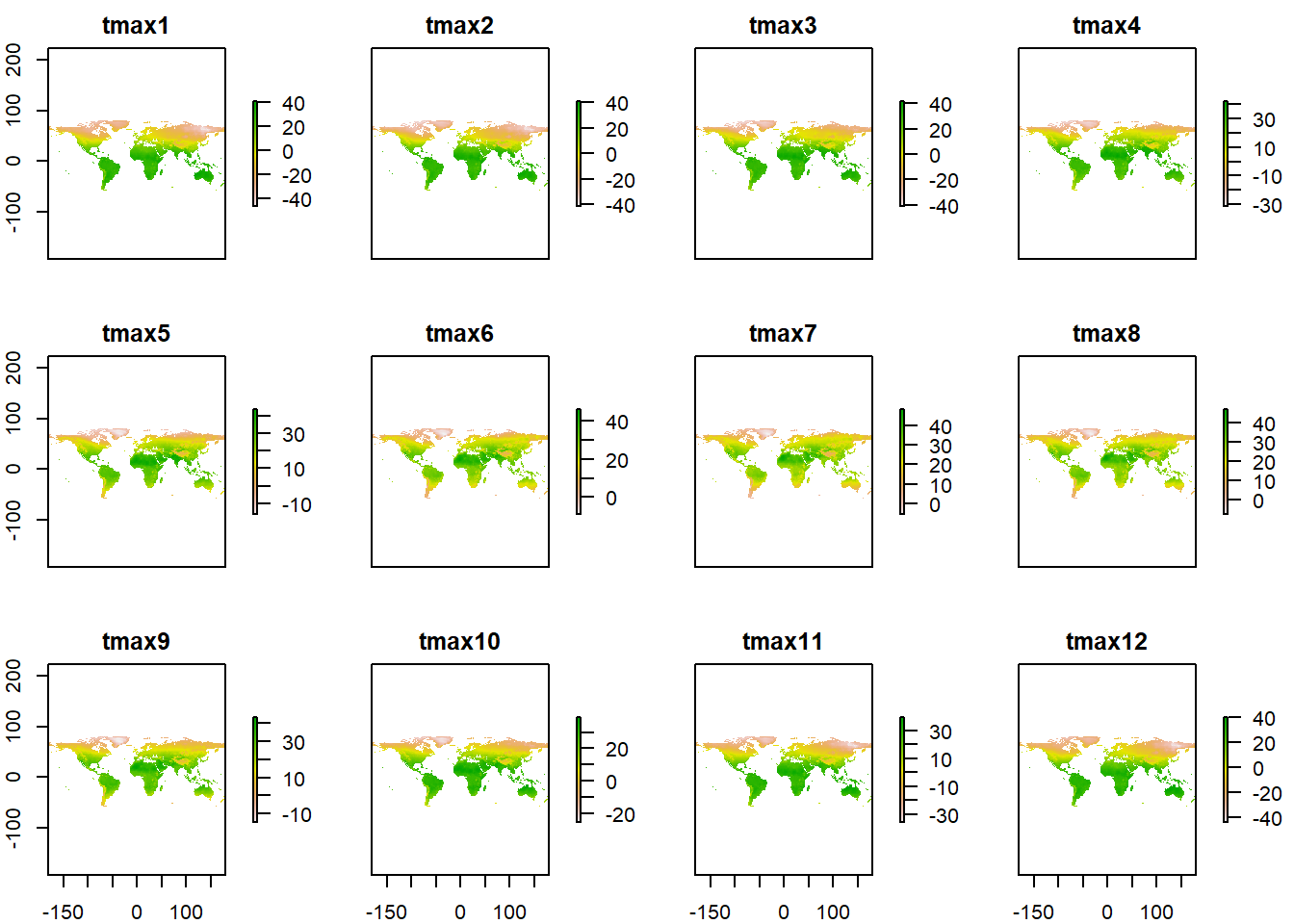
Though the base plot is sharp and quick to draw this large dataset, but we are satisfied with default plotting settings. We can customize the plot and make them appeal to the eye, but we switch to ggplot2 package (Wickham 2016), which does have tons of tools for customization of publication quality plots. Unfortunate, ggplot2 require tidy data in data frame format instead of the raster. Therefore, the first thing is to convert raster to a data frame, the chunk bleow highlihgth.
tmax.tb = tmax %>%
  raster::as.data.frame(xy = TRUE) %>%
  pivot_longer(cols = 3:14, values_to = "tmax", names_to = "month")

tmax.tb
# A tibble: 23,328,000 x 4
x y month tmax
<dbl> <dbl> <chr> <dbl>
1 -180. 89.9 tmax1 NA
2 -180. 89.9 tmax2 NA
3 -180. 89.9 tmax3 NA
4 -180. 89.9 tmax4 NA
5 -180. 89.9 tmax5 NA
6 -180. 89.9 tmax6 NA
7 -180. 89.9 tmax7 NA
8 -180. 89.9 tmax8 NA
9 -180. 89.9 tmax9 NA
10 -180. 89.9 tmax10 NA
# ... with 23,327,990 more rowsOnce we have the data converted to data frame, we can use the power of ggplot2 to visualize land surface maximum temperature at global level by months as highlighted below.
ggplot() +
  geom_raster(data = tmax.tb, aes(x = x, y = y, fill = tmax)) +
  facet_wrap(~month)+
  scale_fill_gradientn(colours = oce::oce.colors9A(120), na.value = NA)+
  theme(panel.background = element_blank(),
        strip.background = element_blank(),
        axis.title = element_blank())+
  scale_x_continuous(breaks = seq(-100,100,100), labels = metR::LonLabel(seq(-100,100,100)))+
  scale_y_continuous(breaks = seq(-50,50,50), labels = metR::LatLabel(seq(-50,50,50)))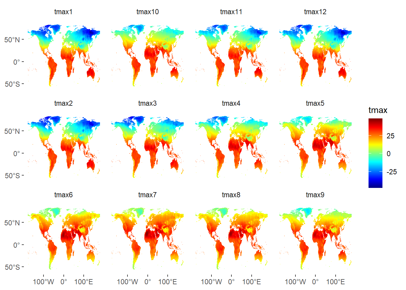
Figure 1: Global land surface temperature by months
We notice that although facet_wrap function plotted figure 1 well and the variation in temperature is visible, but the order of months follow the alphabetic and rather month’s ascending order. We need to tweek around the order. As a first step, we have to reorder the levels of our grouping variable using the level function:
tmax.tb.order = tmax.tb %>%
  mutate(group = factor(x = month, levels = month.abb))
Now, we can draw our plot again:
ggplot() +
  geom_raster(data = tmax.tb.order, aes(x = x, y = y, fill = tmax)) +
  facet_wrap(~group)+
  scale_fill_gradientn(colours = oce::oce.colors9A(120), na.value = NA)+
  theme(panel.background = element_blank(),
        strip.background = element_blank(),
        axis.title = element_blank())+
  scale_x_continuous(breaks = seq(-100,100,100), labels = metR::LonLabel(seq(-100,100,100)))+
  scale_y_continuous(breaks = seq(-50,50,50), labels = metR::LatLabel(seq(-50,50,50)))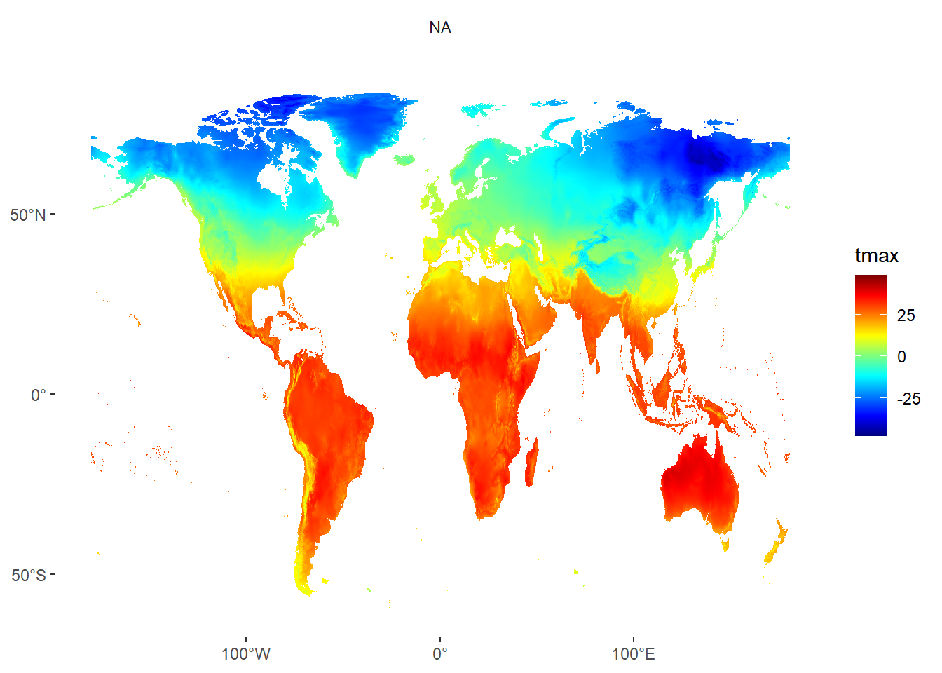
Figure 2: Global land surface temperature by months
Figure 2 shows the output of the reordered facet plot created with the ggplot2.
save the file
Once we are happy with the data we have downloaded and cleaned up, we can now save it into our directory for future use. We do that using a writeRaster from raster package and specify the the file object and the filename as the chunk highlight
tmax %>%
  raster::writeRaster(filename = "wcData/tmax_hist.tif")
Minitmum Temperature
tmin = raster::getData(name = 'worldclim',
                       var = 'tmin',
                       res = 10)
Precipitation
prec = raster::getData(name = 'worldclim',
                       var = 'prec',
                       res = 10)
Bioclimatic variables
Bioclimatic variables are derived from the monthly temperature and rainfall values in order to generate more biologically meaningful variables. These are often used in species distribution modeling and related ecological modeling techniques. The bioclimatic variables represent annual trends (e.g., mean annual temperature, annual precipitation) seasonality (e.g., annual range in temperature and precipitation) and extreme or limiting environmental factors (e.g., temperature of the coldest and warmest month, and precipitation of the wet and dry quarters). The list of all derived bio–climatic variable is shown in table 1.
| Code | Description |
|---|---|
| BIO1 | Annual Mean Temperature |
| BIO2 | Mean Diurnal Range (Mean of monthly (max temp - min temp)) |
| BIO3 | Isothermality (BIO2/BIO7) (<d7>100) |
| BIO4 | Temperature Seasonality (standard deviation <d7>100) |
| BIO5 | Max Temperature of Warmest Month |
| BIO6 | Min Temperature of Coldest Month |
| BIO7 | Temperature Annual Range (BIO5-BIO6) |
| BIO8 | Mean Temperature of Wettest Quarter |
| BIO9 | Mean Temperature of Driest Quarter |
| BIO10 | Mean Temperature of Warmest Quarter |
| BIO11 | Mean Temperature of Coldest Quarter |
| BIO12 | Annual Precipitation |
| BIO13 | Precipitation of Wettest Month |
| BIO14 | Precipitation of Driest Month |
| BIO15 | Precipitation Seasonality (Coefficient of Variation) |
| BIO16 | Precipitation of Wettest Quarter |
| BIO17 | Precipitation of Driest Quarter |
| BIO18 | Precipitation of Warmest Quarter |
| BIO19 | Precipitation of Coldest Quarter |
bio = raster::getData(name = 'worldclim', var = 'bio', res = 10)bio[[3]] %>% raster::plot(main = "Isothermality ")bio %>%
raster::writeRaster(filename = "wcData/bio_hist.tif")Future Climate Data
To get (projected) future climate data (CMIP5), we must provide arguments var and res as above and add model, rcp and year arguments. Only resolutions 2.5, 5, and 10 are currently available. For example, I am interested with the world feature maximum temperature
tmax_future = raster::getData('CMIP5', var='tmax', res=10, rcp=85, model='AC', year=70)

names(tmax_future) = c("Jan", "Feb", "Mar", "Apr", "May", "Jun", "Jul", "Aug", "Sep", "Oct", "Nov", "Dec")