
Data types in R
R is a flexible language that allows to work with different kind of data format [@bradley]. This inluced integer, numeric, character, complex, dates and logical. The default data type or class in R is double precision—numeric. In a nutshell, R treats all kind of data into five categories but we deal with only four in this book. Before proceeding, we need to clear the workspace by typing rm(list = ls()) after the prompt in the in a console.
But before we move further, let’s us clean our working environment by clicking a combination of Ctrl+L. Clearing the workspace is always recommended before working on a new R project to avoid name conflicts with provious projects. We can also clear all figures using graphics.off() function. It is a good code practise that a new R project start with the code in the chunk below:
rm(list = ls())
graphics.off()Integers:Integer values do not have decimal places. They are commonly used for counting or indexing.
aa = c(20,68,78,50)You can check if the data is integer with is.integer() and can convert numeric value to an integer with as.integer()
is.integer(aa)FALSE [1] FALSEYou can query the class of the object with the class() to know the class of the object
class(aa)FALSE [1] "numeric"Although the object bb is integer as confirmed with as.integer() function, the class() ouput the answer as numeric. This is because the defaul type of number in r is numeric. However, you can use the function as.integer() to convert numeric value to integer
class(as.integer(aa))FALSE [1] "integer"Numeric: The numeric class holds the set of real numbers — decimal place numbers. The numeric class is more general than the integer class, and inclused the integer numbers.
These could be any number (whole or decimal number). You can check if the data is integer with is.integer()
bb = c(12.5, 45.68, 2.65)
class(bb)
FALSE [1] "numeric"is.numeric(bb)FALSE [1] TRUEStrings: In programming terms, we usually call text as string.This often aretextdata like names.
countries = c("Kenya", "Uganda", "Rwanda", "Tanzania")
class(countries)
FALSE [1] "character"We can be sure whether the object is a string with is.character() or check the class of the object with class().
Factor: These are strings from finite set of values. For example, we might wish to store a variable that records gender of people. You can check if the data is factor withis.factor()and useas.factor()to convertstringtofactor
sex = c("Male", "Female", "Male", "Male", "Female")
sex = as.factor(sex)
class(sex)
FALSE [1] "factor"Often times we need to know the possible groups that are in the factor data. This can be achieved with the levels() function
levels(sex)FALSE [1] "Female" "Male"levels(countries)FALSE NULLOften we wish to take a continuous numerical vector and transform it into a factor. The function cut() takes a vector of numerical data and creates a factor based on your give cut-points. Let us make a fictional income of 508 people with rnorm() function.
income = rnorm(n = 508, mean = 500, sd = 80)
hist(income, col = "green", main = "", las = 1, xlab = "Individual Income")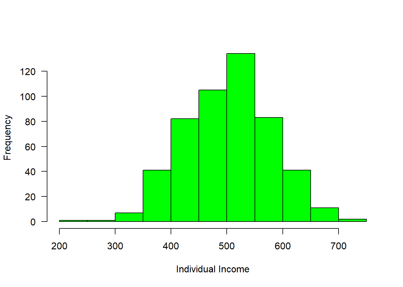
Figure 1: Income distribution
#mosaic::plotDist(dist = "norm", mean = 500, sd = 80)We can now breaks the distribution into groups and make a simple plot as shown in figure 2, where those with income less than 400 were about 50, followed with a group with income range between 400 and 500 of about 200 and 250 people receive income above 500
group = cut(income, breaks = c(300,400,500,800),
            labels = c("Below 400", "400-500", "Above 500"))
is.factor(group)
FALSE [1] TRUElevels(group)FALSE [1] "Below 400" "400-500" "Above 500"barplot(table(group), las = 1, horiz = FALSE, col = c("blue", "red", "blue"), ylab = "Frequency", xlab = "Group of Income")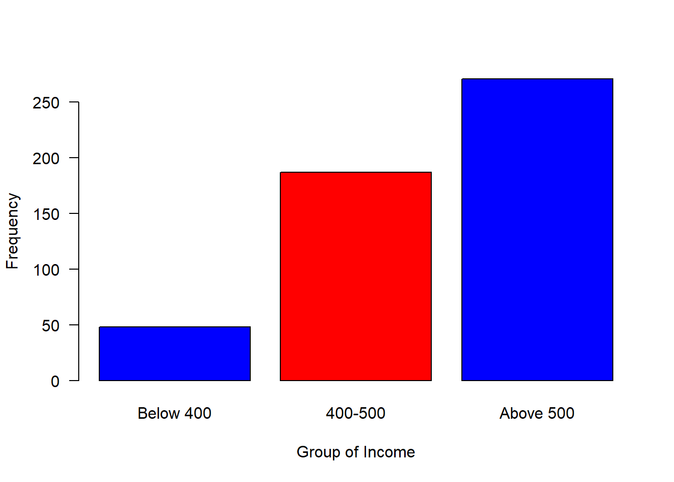
Figure 2: Barplot of grouped income
data = data.frame(group, income)Logicals: This is a special case of a factor that can only take on the valuesTRUEandFALSE. R is case-sensitive, therefore you must always capitalizeTRUEandFALSEin function in R.Date and time
Vectors
Ofen times we want to store a set of numbers in once place. One way to do this is using the vectors in R. Vectors store severl numbers– a set of numbers in one container. let us look on the example below
id = c(1,2,3,4,5)
people = c(158,659,782,659,759)
street = c("Dege", "Mchikichini", "Mwembe Mdogo", "Mwongozo",  "Cheka")
Notice that the c() function, which is short for concatenate wraps the list of numbers. The c() function combines all numbers together into one container. Notice also that all the individual numbers are separated with a comma. The comma is reffered to an an item-delimiter. It allows R to hold each of the numbers separately. This is vital as without the item-delimiter, R will treat a vector as one big, unsperated number.
Indexing the element
One advantage of vector is that you can extract individual element in the vector object by indexing, which is accomplished using the square bracket as illustrated below.
id[5]FALSE [1] 5people[5]FALSE [1] 759street[5]FALSE [1] "Cheka"Apart from extracting single element, indexing allows to extract a range of element in a vector. This is extremely important because it allows to subset a portion of data in a vector. A colon operator is used to extract a range of data
street[2:4]FALSE [1] "Mchikichini" "Mwembe Mdogo" "Mwongozo"Adding and Replacing an element in a vector
It is possible to add element of an axisting vecor. Here ia an example
id[6] = 6
people[6] = 578
street[6] = "Mwongozo"
Sometimes you may need to replace an element from a vector, this can be achieved with indexing
people[1] = 750Number of elements in a vector
Sometimes you may have a long vector and want to know the numbers of elements in the object. R has length() function that allows you to query the vector and print the answer
length(people)FALSE [1] 6Generating sequence of vectors Numbers
There are few R operators that are designed for creating vecor of non-random numbers. These functions provide multiple ways for generating sequences of numbers
The colon : operator, explicitly generate regular sequence of numbers between the lower and upper boundary numbers specified. For example, generating number beween 0 and 10, we simply write;
vector.seq = 0:10
vector.seq
FALSE [1] 0 1 2 3 4 5 6 7 8 9 10However, if you want to generate a vector of sequence number with specified interval, let say we want to generate number between 0 and 10 with interval of 2, then the seq() function is used
regular.vector = seq(from = 0,to = 10, by = 2)
regular.vector
FALSE [1] 0 2 4 6 8 10unlike the seq() function and : operator that works with numbers, the rep() function generate sequence of repeated numbers or strings to create a vector
id = rep(x = 3, each = 4)
station = rep(x = "Station1", each = 4)
id;station
FALSE [1] 3 3 3 3FALSE [1] "Station1" "Station1" "Station1" "Station1"The rep() function allows to parse each and times arguments. The each argument allows creation of vector that that repeat each element in a vector according to specified number.
sampled.months = c("January", "March", "May")
rep(x = sampled.months, each = 3)
FALSE [1] "January" "January" "January" "March" "March" "March" "May"
FALSE [8] "May" "May"But the times argument repeat the whole vector to specfied times
rep(x = sampled.months, times = 3)FALSE [1] "January" "March" "May" "January" "March" "May" "January"
FALSE [8] "March" "May"Generating vector of normal distribution
The central limit theorem that ensure the data is normal distributed is well known to statistician. R has a rnorm() function which makes vector of normal distributed values. For example to generate a vector of 40 sea surface temperature values from a normal distribution with a mean of 25, and standard deviation of 1.58, we simply type this expression in console;
sst = rnorm(n = 40, mean = 25,sd = 1.58)
sst
FALSE [1] 24.03922 23.80315 23.47413 26.27077 23.42572 23.75998 23.61258 23.35309
FALSE [9] 24.69700 22.76580 24.71677 23.02477 27.00590 23.95165 26.52619 26.29226
FALSE [17] 25.35510 24.18597 27.37901 24.34999 24.38044 26.92839 21.37074 25.54579
FALSE [25] 26.55608 26.61256 25.71027 29.16311 25.19961 24.32504 26.28006 25.61089
FALSE [33] 24.85534 24.80107 25.56271 27.84438 24.39485 27.66808 25.80105 24.16359Rounding off numbers
There are many ways of rounding off numerical number to the nearest integers or specify the number of decimal places. the code block below illustrate the common way to round off:
require(magrittr)
chl = rnorm(n = 20, mean = .55, sd = .2)
chl %>% round(digits = 2)
FALSE [1] 0.43 0.58 0.18 0.55 0.85 0.38 0.38 0.40 0.60 0.20 0.74 0.44 0.75 0.37 0.72
FALSE [16] 0.83 0.54 0.53 0.61 0.51Data Frame
data.frame is very much like a simple Excel spreadsheet where each column represents a variable type and each row represent observations. A data frame is the most common way of storing data in R and, generally, is the data structure most often used for data analyses. A data frame is a list of equal–length vectors with rows as records and columns as variables. This makes data frames unique in data storing as it can store different classes of objects in each column (i.e. numeric, character, factor, logic, etc). In this section, we will create data frames and add attributes to data frames.
Creating data frames
Perhaps the easiest way to create a data frame is to parse vectors in a data.frame() function. For instance, in this case we create a simple data frame dt and assess its internal structure
# create vectors
Name  = c('Bob','Jeff','Mary')
Score = c(90, 75, 92)
Grade = c("A", "B", "A")

## use the vectors to make a data frame
dt = data.frame(Name, Score, Grade)

## assess the internal structure
str(dt)
FALSE 'data.frame': 3 obs. of 3 variables:
FALSE $ Name : chr "Bob" "Jeff" "Mary"
FALSE $ Score: num 90 75 92
FALSE $ Grade: chr "A" "B" "A"Note how Variable Name in dt was converted to a column of factors . This is because there is a default setting in data.frame() that converts character columns to factors . We can turn this off by setting the stringsAsFactors = FALSE argument:
## use the vectors to make a data frame
df = data.frame(Name, Score, Grade, stringsAsFactors = FALSE)
df %>% str()
FALSE 'data.frame': 3 obs. of 3 variables:
FALSE $ Name : chr "Bob" "Jeff" "Mary"
FALSE $ Score: num 90 75 92
FALSE $ Grade: chr "A" "B" "A"Now the variable Name is of character class in the data frame. The inherited problem of data frame to convert character columns into a factor is resolved by introduction f advanced data frames called tibble, which provides sticker checking and better formating than the traditional data.frame.
## use the vectors to make a tibble
tb = tibble(Name, Score, Grade)
## check the internal structure of the tibble
tb%>% glimpse()
FALSE Rows: 3
FALSE Columns: 3
FALSE $ Name <chr> "Bob", "Jeff", "Mary"
FALSE $ Score <dbl> 90, 75, 92
FALSE $ Grade <chr> "A", "B", "A"Table 1 show the the data frame created by fusing the two vectors together.
| Name | Score | Grade |
|---|---|---|
| Bob | 90 | A |
| Jeff | 75 | B |
| Mary | 92 | A |
Because the columns have meaning and we have given them column names, it is desirable to want to access an element by the name of the column as opposed to the column number.In large Excel spreadsheets I often get annoyed trying to remember which column something was. The $sign and []are used in R to select variable from the data frame.
dt$NameFALSE [1] "Bob" "Jeff" "Mary"dt[,1]FALSE [1] "Bob" "Jeff" "Mary"dt$ScoreFALSE [1] 90 75 92dt[,2]FALSE [1] 90 75 92R has build in dataset that we can use for illustration. For example, @longley created a longley dataset, which is data frame with 7 economic variables observed every year from 1947 ti 1962 (Table 2). We can add the data in the workspace with data() function
data(longley)

longley %>%
  kable(caption = "Longleys' Economic dataset", align = "c", row.names = F) %>%
column_spec(1:7, width = "3cm")| GNP.deflator | GNP | Unemployed | Armed.Forces | Population | Year | Employed |
|---|---|---|---|---|---|---|
| 83.0 | 234.289 | 235.6 | 159.0 | 107.608 | 1947 | 60.323 |
| 88.5 | 259.426 | 232.5 | 145.6 | 108.632 | 1948 | 61.122 |
| 88.2 | 258.054 | 368.2 | 161.6 | 109.773 | 1949 | 60.171 |
| 89.5 | 284.599 | 335.1 | 165.0 | 110.929 | 1950 | 61.187 |
| 96.2 | 328.975 | 209.9 | 309.9 | 112.075 | 1951 | 63.221 |
| 98.1 | 346.999 | 193.2 | 359.4 | 113.270 | 1952 | 63.639 |
| 99.0 | 365.385 | 187.0 | 354.7 | 115.094 | 1953 | 64.989 |
| 100.0 | 363.112 | 357.8 | 335.0 | 116.219 | 1954 | 63.761 |
| 101.2 | 397.469 | 290.4 | 304.8 | 117.388 | 1955 | 66.019 |
| 104.6 | 419.180 | 282.2 | 285.7 | 118.734 | 1956 | 67.857 |
| 108.4 | 442.769 | 293.6 | 279.8 | 120.445 | 1957 | 68.169 |
| 110.8 | 444.546 | 468.1 | 263.7 | 121.950 | 1958 | 66.513 |
| 112.6 | 482.704 | 381.3 | 255.2 | 123.366 | 1959 | 68.655 |
| 114.2 | 502.601 | 393.1 | 251.4 | 125.368 | 1960 | 69.564 |
| 115.7 | 518.173 | 480.6 | 257.2 | 127.852 | 1961 | 69.331 |
| 116.9 | 554.894 | 400.7 | 282.7 | 130.081 | 1962 | 70.551 |
Sometimes you may need to create set of values and store them in vectors, then combine the vectors into a data frame. Let us see how this can be done. First create three vectors. One contains id for ten individuals, the second vector hold the time each individual signed in the attendane book and the third vector is the distance of each individual from office. We can concatenate the set of values to make vectors.
id  = c(1,2,3,4,5,6,7,8,9,10)

time = ymd_hms(c("2018-11-20 06:35:25 EAT", "2018-11-20 06:52:05 EAT",
                 "2018-11-20 07:08:45 EAT", "2018-11-20 07:25:25 EAT",
                 "2018-11-20 07:42:05 EAT", "2018-11-20 07:58:45 EAT",
                 "2018-11-20 08:15:25 EAT", "2018-11-20 08:32:05 EAT",
                 "2018-11-20 08:48:45 EAT", "2018-11-20 09:05:25 EAT"), tz = "")

distance = c(20, 85, 45, 69, 42,  52, 6, 45, 36, 7)
Once we have the vectors that have the same length dimension, we can use the function data.frame() to combine the the three vectors into one data frame shown in table 3
arrival = data.frame(id, time, distance)| IDs | Time | Distance |
|---|---|---|
| 1 | 2018-11-20 06:35:25 | 20 |
| 2 | 2018-11-20 06:52:05 | 85 |
| 3 | 2018-11-20 07:08:45 | 45 |
| 4 | 2018-11-20 07:25:25 | 69 |
| 5 | 2018-11-20 07:42:05 | 42 |
| 6 | 2018-11-20 07:58:45 | 52 |
| 7 | 2018-11-20 08:15:25 | 6 |
| 8 | 2018-11-20 08:32:05 | 45 |
| 9 | 2018-11-20 08:48:45 | 36 |
| 10 | 2018-11-20 09:05:25 | 7 |
Matrix
A matrix is defined as a collection of data elements arranged in a two–dimensional rectangular layout. R is very strictly when you make up a matrix as it must be with equal dimension—all columns in a matrix must be of the same length. Unlike data frame and list that can store numeric or character.etc in columns, matrix columns must be numeric or characters in a matrix file.
Creating Matrices
The base R has a matrix() function that construct matrices column–wise. In other language, element in matrix are entered starting from the upper left corner and running down the columns. Therefore, one should take serious note of specifying the value to fill in a matrix and the number of rows and columns when using the matrix() function.For example in the code block below, we create an imaginary month sst value for five years and obtain an atomic vector of 60 observation.
sst = rnorm(n = 60, mean = 25, 3)Once we have the atomic vector of sst value, we can convert it to matrix with the matrix() function. We put the observation as rows—months and the columns as years. Therefore, we have 12 rows and 5 years and the product of number of months and years we get 60—equivalent to our sst atomic vector we just created above.
sst.matrix = matrix(data = sst, nrow = 12, ncol = 5)We then check whether we got the matrix with is.matrix() function
is.matrix(sst);is.matrix(sst.matrix)FALSE [1] FALSEFALSE [1] TRUEsstFALSE [1] 25.08327 24.09097 26.34485 24.14146 24.64941 26.09739 23.91218 26.91260
FALSE [9] 22.69753 24.84250 24.89610 21.91391 30.20031 22.91143 26.33853 24.99629
FALSE [17] 23.69466 30.10935 25.78983 25.05814 26.59829 26.77820 26.60457 27.57653
FALSE [25] 24.65990 26.95125 29.67351 20.43879 30.49668 25.97459 24.28109 25.72646
FALSE [33] 21.91946 21.91512 24.87088 27.31100 28.64027 26.58810 27.33460 21.98717
FALSE [41] 29.04679 25.85037 22.84274 22.30848 28.18201 25.51643 29.05196 24.12477
FALSE [49] 19.98520 30.13661 26.37739 25.49994 22.78731 25.80078 23.99339 23.64162
FALSE [57] 26.40151 29.94575 26.80928 23.84312We can check whether the dimension we just defined while creating this matrix is correct. This is done with the dim() function from base R.
dim(sst.matrix)FALSE [1] 12 5If you have large vector and you you want the matrix() function to figure out the number of columns, you simply define the nrow and tell the function that you do not want those element arranged by rows —i.e you want them in column-wise. That is done by parsing the argument byrow = FALSE inside the matrixt() function.
sst.matrixby = sst %>% matrix(nrow = 12, byrow = FALSE)Adding attributes to Matrices
Often times you may need to add additional attributes to the maxtrix—observation names, variable names and comments in the matrix.
We can add columns, which are years from 2014 to 2018
years = 2014:2018
colnames(sst.matrix) = years
sst.matrix
FALSE 2014 2015 2016 2017 2018
FALSE [1,] 25.08327 30.20031 24.65990 28.64027 19.98520
FALSE [2,] 24.09097 22.91143 26.95125 26.58810 30.13661
FALSE [3,] 26.34485 26.33853 29.67351 27.33460 26.37739
FALSE [4,] 24.14146 24.99629 20.43879 21.98717 25.49994
FALSE [5,] 24.64941 23.69466 30.49668 29.04679 22.78731
FALSE [6,] 26.09739 30.10935 25.97459 25.85037 25.80078
FALSE [7,] 23.91218 25.78983 24.28109 22.84274 23.99339
FALSE [8,] 26.91260 25.05814 25.72646 22.30848 23.64162
FALSE [9,] 22.69753 26.59829 21.91946 28.18201 26.40151
FALSE [10,] 24.84250 26.77820 21.91512 25.51643 29.94575
FALSE [11,] 24.89610 26.60457 24.87088 29.05196 26.80928
FALSE [12,] 21.91391 27.57653 27.31100 24.12477 23.84312and add the month for rows, which is January to December. Now the matrix has names for the rows—records and for columns—variables
months = seq(from = dmy(010115), to = dmy(311215),
             by = "month") %>% month(abbr = TRUE,
                                     label = TRUE)
rownames(sst.matrix) = months
sst.matrix
FALSE 2014 2015 2016 2017 2018
FALSE Jan 25.08327 30.20031 24.65990 28.64027 19.98520
FALSE Feb 24.09097 22.91143 26.95125 26.58810 30.13661
FALSE Mar 26.34485 26.33853 29.67351 27.33460 26.37739
FALSE Apr 24.14146 24.99629 20.43879 21.98717 25.49994
FALSE May 24.64941 23.69466 30.49668 29.04679 22.78731
FALSE Jun 26.09739 30.10935 25.97459 25.85037 25.80078
FALSE Jul 23.91218 25.78983 24.28109 22.84274 23.99339
FALSE Aug 26.91260 25.05814 25.72646 22.30848 23.64162
FALSE Sep 22.69753 26.59829 21.91946 28.18201 26.40151
FALSE Oct 24.84250 26.77820 21.91512 25.51643 29.94575
FALSE Nov 24.89610 26.60457 24.87088 29.05196 26.80928
FALSE Dec 21.91391 27.57653 27.31100 24.12477 23.84312Arrays
array(data = sst, dim = c(3,5,4))FALSE , , 1
FALSE
FALSE [,1] [,2] [,3] [,4] [,5]
FALSE [1,] 25.08327 24.14146 23.91218 24.84250 30.20031
FALSE [2,] 24.09097 24.64941 26.91260 24.89610 22.91143
FALSE [3,] 26.34485 26.09739 22.69753 21.91391 26.33853
FALSE
FALSE , , 2
FALSE
FALSE [,1] [,2] [,3] [,4] [,5]
FALSE [1,] 24.99629 25.78983 26.77820 24.65990 20.43879
FALSE [2,] 23.69466 25.05814 26.60457 26.95125 30.49668
FALSE [3,] 30.10935 26.59829 27.57653 29.67351 25.97459
FALSE
FALSE , , 3
FALSE
FALSE [,1] [,2] [,3] [,4] [,5]
FALSE [1,] 24.28109 21.91512 28.64027 21.98717 22.84274
FALSE [2,] 25.72646 24.87088 26.58810 29.04679 22.30848
FALSE [3,] 21.91946 27.31100 27.33460 25.85037 28.18201
FALSE
FALSE , , 4
FALSE
FALSE [,1] [,2] [,3] [,4] [,5]
FALSE [1,] 25.51643 19.98520 25.49994 23.99339 29.94575
FALSE [2,] 29.05196 30.13661 22.78731 23.64162 26.80928
FALSE [3,] 24.12477 26.37739 25.80078 26.40151 23.84312This can be done with the indexing. For example, in the sst.matrix we just create, it has twelve rows representing monthly average and five columns representing years. We then obtain data for the six year and we want to add it into the matrix. Simply done with indexing
sst.matrix[1:12,5]FALSE Jan Feb Mar Apr May Jun Jul Aug
FALSE 19.98520 30.13661 26.37739 25.49994 22.78731 25.80078 23.99339 23.64162
FALSE Sep Oct Nov Dec
FALSE 26.40151 29.94575 26.80928 23.84312Dealing with Misiing Values
Just as we can assign numbers, strings, list to a variable, we can also assign nothing to an object, or an empty value to a variable. IN R, an empty object is defined with NULL. Assigning a value oof NULL to an object is one way to reset it to its original, empty state. You might do this when you wanto to pre–allocate an object without any value, especially when you iterate the process and you want the outputs to be stored in the empty object.
sst.container = NULLYou can check whether the object is an empty with the is.null() function, which return a logical ouputs indicating whther is TRUE or FALSE
is.null(sst.container)FALSE [1] TRUEYou can also check for NULL in an if satement as well, as highlighted in the following example;
if (is.null(sst.container)){
  print("The object is empty and hence you can use to store looped outputs!!!")
}
FALSE [1] "The object is empty and hence you can use to store looped outputs!!!"And empty element (value) in object is represented with NA in R, and it is the absence of value in an object or variable.
sst.sample = c(26.78, 25.98,NA, 24.58, NA)
sst.sample
FALSE [1] 26.78 25.98 NA 24.58 NATo identify missing values in a vector in R, use the is.na() function, which returns a logical vector with TRUE of the corresponding element(s) with missing value
is.na(sst.sample)FALSE [1] FALSE FALSE TRUE FALSE TRUEand computing statistics of the variable with NA always will give out the NA ouputs
mean(sst.sample); sd(sst.sample);range(sst.sample)FALSE [1] NAFALSE [1] NAFALSE [1] NA NAHowever, we can exclude missing value in these mathematical operations by parsing , na.rm = TRUE argument
mean(sst.sample, na.rm = TRUE);sd(sst.sample, na.rm = TRUE);range(sst.sample, na.rm = TRUE)FALSE [1] 25.78FALSE [1] 1.113553FALSE [1] 24.58 26.78you can also exclude the element with NA value using the `na.omit()
sst.sample %>% na.omit()FALSE [1] 26.78 25.98 24.58
FALSE attr(,"na.action")
FALSE [1] 3 5
FALSE attr(,"class")
FALSE [1] "omit"Finally is a NaN, which is closely related to NA, which is used to assign non-floating numbers. For example when we have the anomaly of sea surface temperature and we are interested to use sqrt() function to reduce the variability of the dataset.
sst.anomaly = c(2.3,1.25,.8,.31,0,-.21)
sqrt(sst.anomaly)
FALSE [1] 1.5165751 1.1180340 0.8944272 0.5567764 0.0000000 NaNWe notice that the sqrt of -0.21 gives us a NaN elements.
