CHIRPS precipitation data made easier access in R with wior package

The Climate Hazards Group InfraRed Precipitation with Station data (CHIRPS) is a quasi-global rainfall data set. As its title suggests it combines data from real-time observing meteorological stations with infra-red satellite data to estimate precipitation. CHIRPS incorporates 0.05° resolution satellite imagery with in-situ station data to create gridded rainfall time series for trend analysis and seasonal drought monitoring.

The global dataset covers the area from \(40^\circ\)N to \(4^\circ\)S and from \(20^\circ\)W to \(50^\circ\)E with a spatial resolution of 0.05\(^\circ\) grid at daily, pentad, monthly and annual time interval. This is equivalent to 5.5 km² grid at the equator spaning from January 1981 to the near present.

Despite the effort of the National Aeronautics and Space Administration (NASA), and the National Oceanic and Atmospheric Administration (NOAA) to developoping techniques for producing global rainfall maps at high spatial and temporal resolution, these datasets are provided in NetCDF, Geotiff and Esri BIL formats. These formats are commonly in science, however, for for scripting programming languages like R and Python, the core format for data analysis and visualizaation are data frames.

In this post, I illustrate how to access chirps data from any area of the earth’s surface using a get_precip function from wior package (Semba and Peter 2020). The package not only download the precipitation data, it also transform and structure the values into a tidy format (Wickham and Henry 2018). According to Wickham and Henry (2018), a tidy data is stored in data frame that adhere to the following three key conditions;

1. each column is a variable
2. each row is an observation
3. each value has its own cell

Once the data is in this format, we can harness the analytical power using severa packages and plotting with popular graphic packages like ggplot2 and metR packages.

We first install the package from github

# install.packages("devtools")
devtools::install_github("lugoga/wior")

Once you have installed the data into your machine, we can download the rainfall data for any place covered by the project. For illustration, I chose to assess the rainfall patterns in the Ukerewe Island, in Lake Victoria. We first load the packages needed for this tasks

require(tidyverse)
require(wior)

We want the monthly data (level = 3) from 1981 to present. The code below highlight the key parameters required in the get_precip function.

ukerewe = wior::get_precip(lon.min = 32.9, 
                           lon.max = 33.14, 
                           lat.min = -2.16,
                           lat.max = -1.96, 
                           t1 = "1981-01-01", 
                           t2 = "2019-12-31", 
                           level = 3)

Once our precipitation data is dowloaded, we can check the first three rows and the last three rows with the FSA package. We notice that the firs rows begin in 01-01-1981 and the last lows is dated on 01-08-2021.

ukerewe %>% FSA::headtail()

            time  latitude longitude   precip
1     1981-01-01 -2.175003  32.87500 63.82610
2     1981-01-01 -2.175003  32.92500 66.01859
3     1981-01-01 -2.175003  32.97499 68.29806
14638 2021-08-01 -1.975002  33.02499 39.38923
14639 2021-08-01 -1.975002  33.07500 32.23105
14640 2021-08-01 -1.975002  33.12500 32.98096

We can then use the ggplot package (Wickham 2016) to compare the spatial distribution of precipitation over the island for over 39 years as shown in figure 1

ukerewe %>% 
  mutate(year = lubridate::year(time)) %>% 
  group_by(latitude,longitude, year) %>% 
  summarise(precip = sum(precip, na.rm = TRUE)) %>% 
  ungroup() %>% 
  ggplot(aes(x = longitude, y = latitude, z = precip))+
  metR::geom_contour_fill(bins = 6, global.breaks = FALSE) + 
  # metR::geom_contour2(breaks = 1200, size = 0.2)+
  facet_wrap(~year)+
  scale_fill_gradientn(colours = mycolor,  name = "Precip \n (mm/year)",
                       trans = scales::boxcox_trans(p = 0.01),
                       breaks = scales::breaks_width(width = 200, offset = -50))+
  scale_x_continuous(breaks = 33, labels = metR::LonLabel(33), expand = c(0,0))+
  scale_y_continuous(breaks = -2.1, labels = metR::LatLabel(-2.1), expand = c(0,0))+
  theme_bw()+
  theme(axis.title = element_blank(), strip.background = element_blank())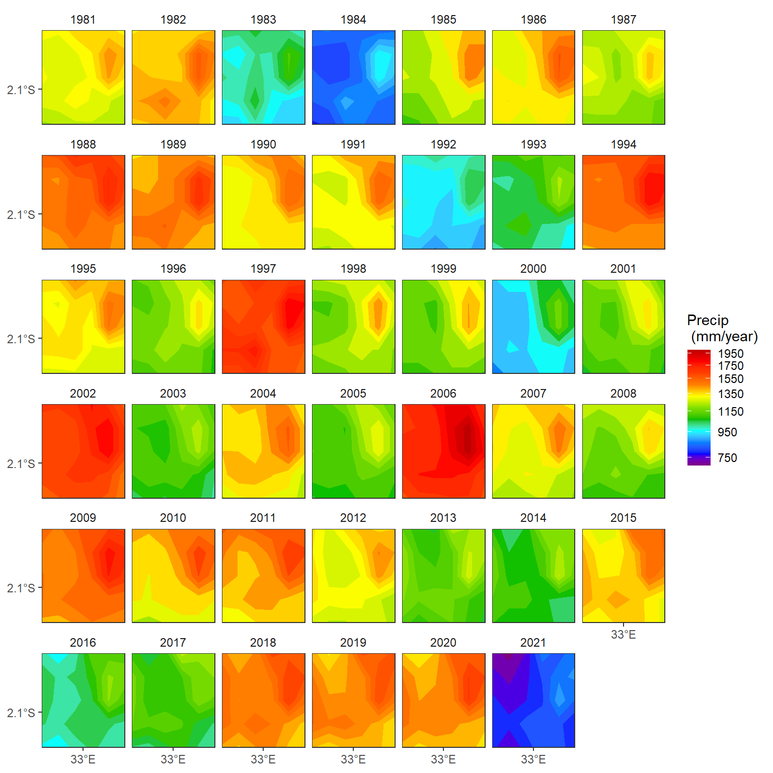

Figure 1: Precipitation patterns in Ukerewe Island