Analyse questionnaire and surveys in R
Introduction
This post offers some technique on how to analyse data from a surveys and questionnaires in R, provides tips on visualizing survey data, and exemplifies how survey and questionnaire data can be analyzed.
Questionnaires and surveys are widely used in research and thus one of the most common research designs. Questionnaires elicit three types of data:
- Factual
- Behavioral
- Attitudinal
While factual and behavioral questions are about what the respondent is and does, attitudinal questions tap into what the respondent thinks or feels.
The advantages of surveys are that they * offer a relative cheap, quick, and effective way to collect (targeted) data from a comparatively large set of people; and * that they can be distributed or carried out in various formats (face-to-face, by telephone, by computer or via social media, or by postal service).
Disadvantages of questionnaires are that they are prone to providing unreliable or unnatural data. Data gathered via surveys can be unreliable due to the social desirability bias which is the tendency of respondents to answer questions in a manner that will be viewed favorably by others. Thus, the data that surveys provide may not necessarily be representative of actual natural behavior.
In this section, we will discuss what needs to kept in mind when designing questionnaires and surveys, what pieces of software or platforms one can use, options for visualizing questionnaire and survey data, statistical methods that are used to evaluate questionnaire and survey data (reliability), and which statistical methods are used in analyzing the data.
packages
s
library(tidyverse)
library(likert)
load the dataset
qns = read_csv("BIOSTATISTIC-Responses.csv")qns %>%
glimpse()Rows: 96
Columns: 24
$ Timestamp <chr> ~
$ `First Name` <chr> ~
$ Surname <chr> ~
$ `Registration Number` <chr> ~
$ `Email address` <chr> ~
$ Gender <chr> ~
$ `What is your body weight (in Kilogram)` <dbl> ~
$ `What is your body Height (in meters)` <dbl> ~
$ `What undergraduate degree programme are you pursuing with at UDOM?` <chr> ~
$ `Looking on yourself, where would you position yourself in the rank below based on the your ability in doing mathematic?` <dbl> ~
$ `Which of the following best describe your objective for taking Biostatistics course` <chr> ~
$ `Do you have access to internet enabled Desktop or Laptop?` <chr> ~
$ `Which subject did you major in your Advanced Level Studies? (Multiple selection)` <chr> ~
$ `What statistical software, if any have you used in the past (multiple selection)` <chr> ~
$ `How interested would you be in the ability to do labwork, exercise and quizzes for this Biostatistics course?` <chr> ~
$ `How interested would you be for group work during the timeflame of this course?` <chr> ~
$ `How interested would you be forming study group with other student?` <chr> ~
$ `When do you typically prefer learning Biostatistics and its application` <chr> ~
$ `What proportion of the time in your semester classes do you spend learning Biostatistics?` <chr> ~
$ `What document formats are you familiar with?` <chr> ~
$ `In your previous Practical Training, did you collect any biological data?` <chr> ~
$ `If the answer is yes, did you analyse the data you collect?` <chr> ~
$ `Which software did you use for the analysis of the data you collected?` <chr> ~
$ `Please let us know of any ideas you might have to improve and enhance better understanding of the Biostatistics course to your fellow students?` <chr> ~Visualizing survey data
Just as the data that is provided by surveys and questionnaires can take various forms, there are numerous ways to display survey data. In the following, we will have a look at some of the most common or useful ways in which survey and questionnaire data can be visualized. However, before we can begin, we need to set up our R session as shown below.
Line graphs for Likert-scaled data
A special case of line graphs is used when dealing with Likert-scaled variables (we will talk about Likert scales in more detail below). In such cases, the line graph displays the density of cumulative frequencies of responses. The difference between the cumulative frequencies of responses displays differences in preferences. We will only focus on how to create such graphs using the ggplot environment here as it has an in-build function (ecdf) which is designed to handle such data.
The questionnaire dataset contains Likert-scaled variables about their competency in using computer. The response to the Likert item is numeric so that very incompetent would get the lowest (1) and high comppetent the highest numeric value (5).
pc = qns %>%
  # glimpse() %>%
  select(degree = 9, competance = 10)

pc
# A tibble: 96 x 2
degree competance
<chr> <dbl>
1 BSc-Biology 5
2 BSc-Biology 5
3 BSc-Biology 2
4 BSc-Biology 3
5 BSc-Biology 2
6 BSc-Biology 4
7 BSc-Biology 4
8 BSc-Biology 4
9 BSc-Biology 4
10 BSc-Biology 2
# ... with 86 more rowsThe pc dataset set has only two columns: a column labeled degree which has three degree programs (German, Japanese, and Chinese) and a column labeled competence which contains values from 1 to 5 which represent values ranging from very incompetent to very competent. Now that we have data resembling a Likert-scaled item from a questionnaire, we will display the data in a cumulative line graph.
pc %>%
  ggplot(aes(x = competance, color = degree))+
  geom_step(aes(y = ..y..), stat = "ecdf")+
  scale_y_continuous(name = "Cumulative Density")+
  scale_x_discrete(limits = c("1","2","3","4","5"),
                   breaks = c(1,2,3,4,5),
                   labels=c("Very incompetent", "Incompetent",
                            "Neutral", "Competent", "Very competent")) +
  ggsci::scale_color_d3()+
  theme_bw() +
  theme(legend.position = c(.12,.85))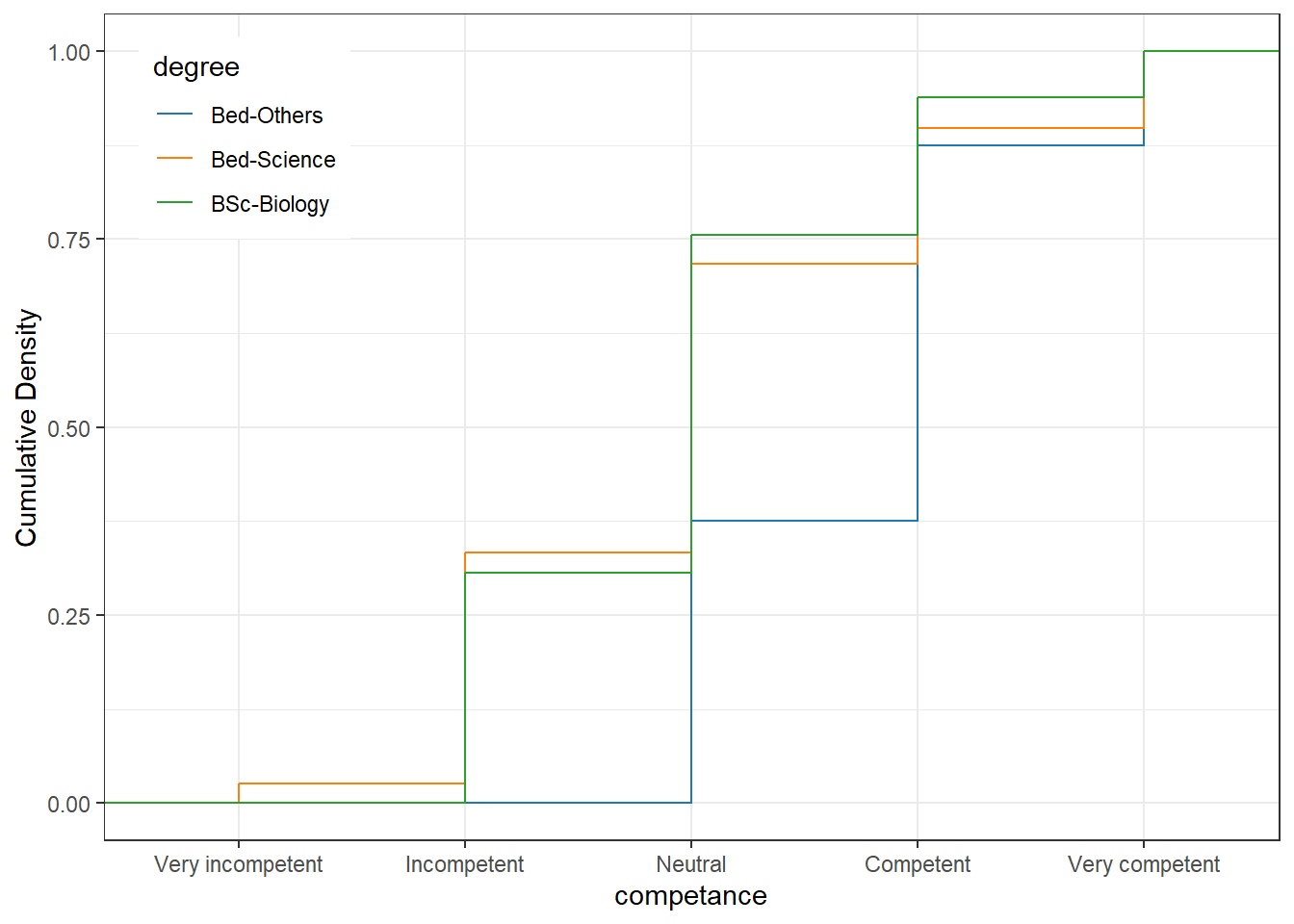
Pie charts
Most commonly, the data for visualization comes from tables of absolute frequencies associated with a categorical or nominal variable. The default way to visualize such frequency tables are pie charts and bar plots. In a first step, we modify the data to get counts and percentages.
degree = qns %>%
  rename(degree = 9) %>%
  group_by(degree) %>%
  summarise(count = n()) %>%
  mutate(percent = count/sum(count)*100,
         across(is.numeric, round, 1)) %>%
  ungroup() %>%
  mutate(degree = if_else(is.na(degree), "Unspecified", degree))


degree
# A tibble: 3 x 3
degree count percent
<chr> <dbl> <dbl>
1 Bed-Others 8 8.3
2 Bed-Science 39 40.6
3 BSc-Biology 49 51 degree %>%
ggplot(aes(x = "", y = percent, fill = degree))+
geom_col(color = "white")+
coord_polar(theta = "y", start = 0)+
theme_void()+
ggsci::scale_fill_d3()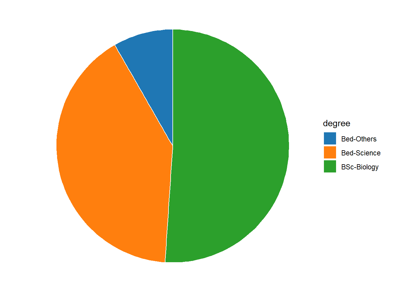
If the slices of the pie chart are not labelled, it is difficult to see which slices are smaller or bigger compared to other slices. This problem can easily be avoided when using a bar plot instead. This issue can be avoided by adding labels to pie charts. The labeling of pie charts is, however, somewhat tedious as the positioning is tricky. Below is an example for adding labels without specification.
degree %>%
  ggplot(aes(x = "", y = percent, fill = degree))+
  geom_col(color = "white")+
  coord_polar(theta = "y", start = 0)+
  geom_text(aes(y = percent, label = percent), color = "white")+
  theme_void()+
  ggsci::scale_fill_d3()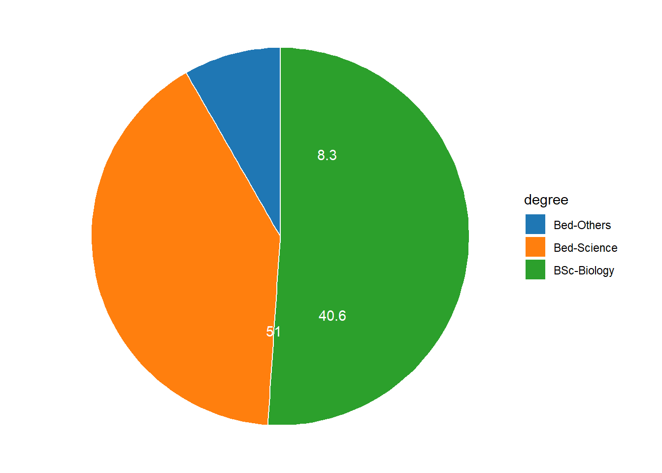
To place the labels where they make sense, we will add another variable to the data called “Position”.
pdegree = degree %>%
  arrange(desc(degree)) %>%
  mutate(position = cumsum(percent) - 0.5*percent)

pdegree
# A tibble: 3 x 4
degree count percent position
<chr> <dbl> <dbl> <dbl>
1 BSc-Biology 49 51 25.5
2 Bed-Science 39 40.6 71.3
3 Bed-Others 8 8.3 95.8Now that we have specified the position, we can include it into the pie chart.
pdegree %>%
  ggplot(aes(x = "", y = percent, fill = degree))+
  geom_col(color = "white")+
  coord_polar(theta = "y", start = 0)+
  geom_text(aes(y = position, label = percent), color = "white")+
  theme_void()+
  ggsci::scale_fill_d3()
We will now create separate pie charts for each gender. In a first step, we create a data set that does not only contain the degree levels and their frequency but also the gender.
degree.gender = qns %>%
  rename(degree = 9, gender = Gender) %>%
  group_by(gender, degree) %>%
  summarise(count = n()) %>%
  mutate(percent = count/sum(count)*100, across(is.numeric, round, 1)) %>%
  arrange(desc(degree)) %>%
  # ungroup() %>%
  mutate(position = cumsum(percent) - 0.5*percent)

degree.gender
# A tibble: 6 x 5
# Groups: gender [2]
gender degree count percent position
<chr> <chr> <dbl> <dbl> <dbl>
1 Female BSc-Biology 12 38.7 19.4
2 Male BSc-Biology 37 56.9 28.4
3 Female Bed-Science 12 38.7 58.0
4 Male Bed-Science 27 41.5 77.6
5 Female Bed-Others 7 22.6 88.7
6 Male Bed-Others 1 1.5 99.2Let’s briefly inspect the new data set. Now that we have created the dataset, we can plot separate pie charts for each gender.
degree.gender %>%
  ggplot(aes(x = "", y = percent, fill = degree))+
  geom_col(color = "white")+
  geom_text(aes(y = position, label = percent), color = "white")+
  facet_wrap(~gender)+
  coord_polar(theta = "y", start = 0)+
  theme_void()+
  ggsci::scale_fill_d3()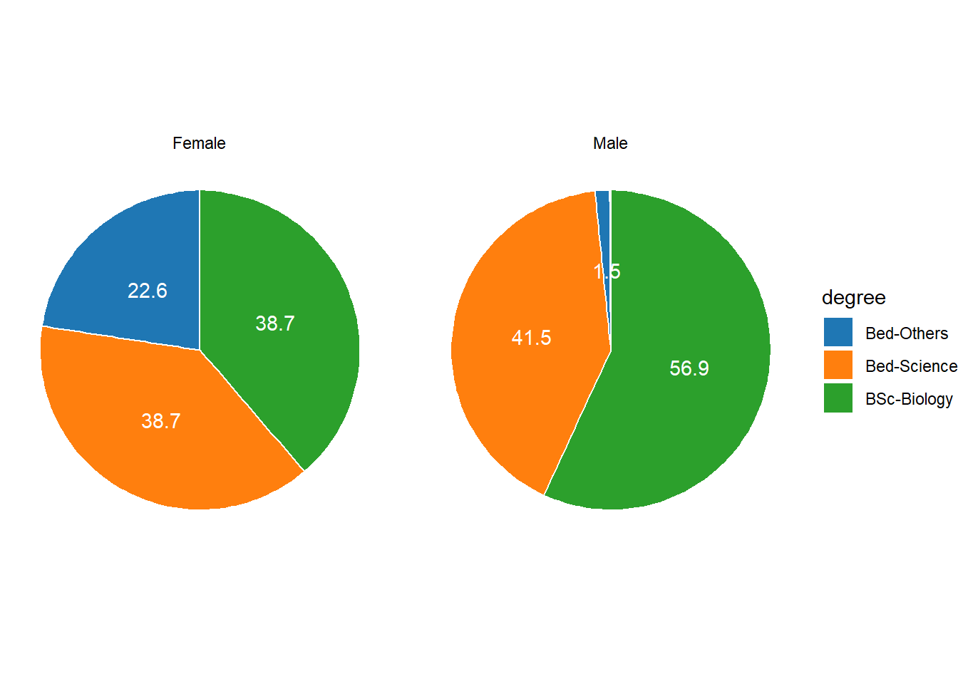
Bar plots
Like pie charts, bar plot display frequency information across categorical variable levels.
degree.count = qns %>%
  select(degree = 9, gender = Gender) %>%
  group_by(degree) %>%
  count()

degree.count
# A tibble: 3 x 2
# Groups: degree [3]
degree n
<chr> <int>
1 Bed-Others 8
2 Bed-Science 39
3 BSc-Biology 49degree.count %>%
ggplot(aes(x = degree, y = n, fill = degree))+
geom_col()+
geom_text(aes(x = degree, y = n-3, label = n), color = "white")+
scale_y_continuous(name = "Frequency", expand = c(0, NA))+
ggsci::scale_fill_d3()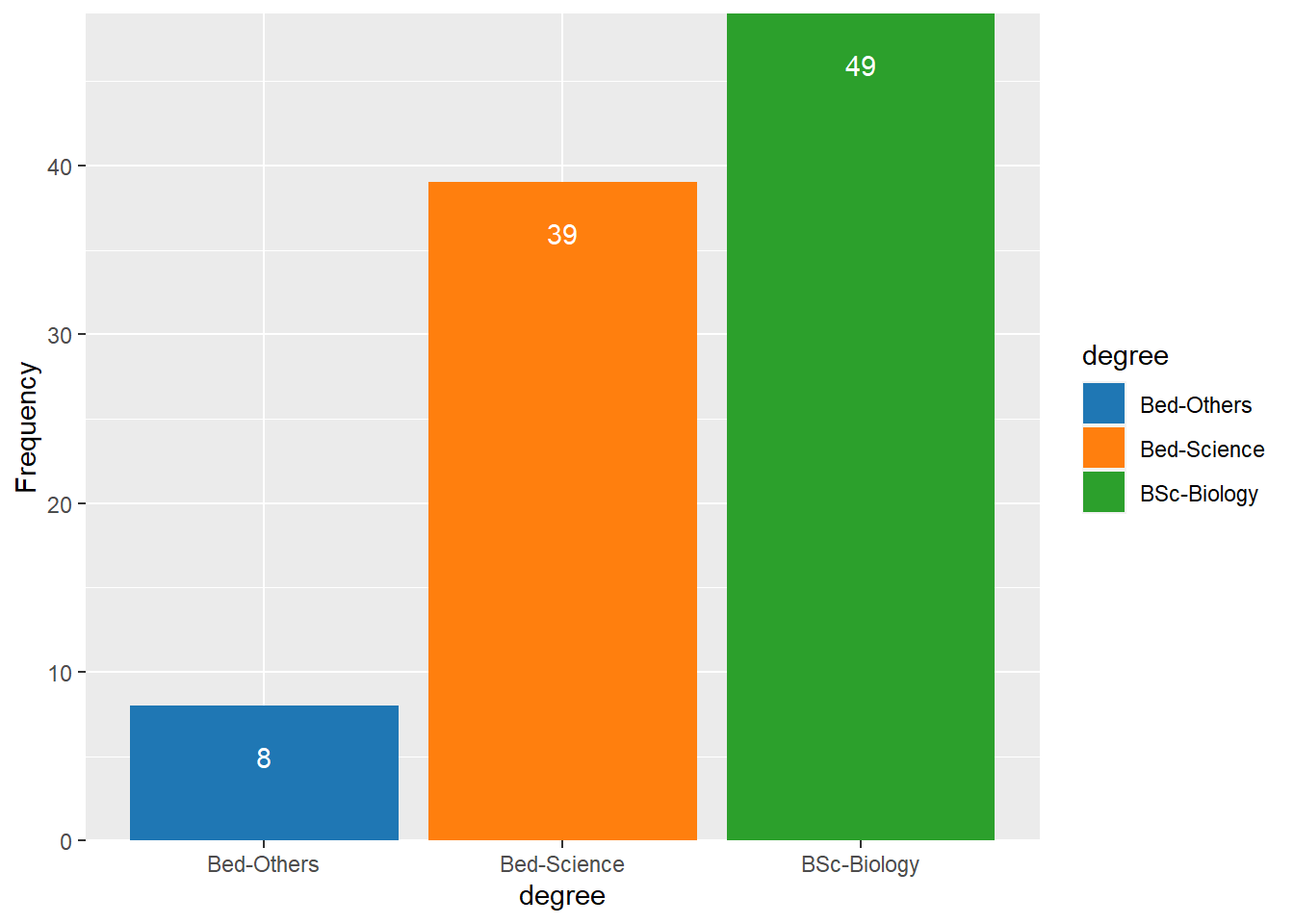
Compared with the pie chart, it is much easier to grasp the relative size and order of the percentage values which shows that pie charts are unfit to show relationships between elements in a graph and, as a general rule of thumb, should be avoided.
Bar plots can be grouped which adds another layer of information that is particularly useful when dealing with frequency counts across multiple categorical variables. But before we can create grouped bar plots, we need to create an appropriate data set.
degree.gender.count = qns %>%
  select(degree = 9, gender = Gender) %>%
  group_by(degree,gender) %>%
  count()

degree.gender.count
# A tibble: 6 x 3
# Groups: degree, gender [6]
degree gender n
<chr> <chr> <int>
1 Bed-Others Female 7
2 Bed-Others Male 1
3 Bed-Science Female 12
4 Bed-Science Male 27
5 BSc-Biology Female 12
6 BSc-Biology Male 37We have now added Course as an additional categorical variable and will include gender as the “fill” argument in our bar plot. To group the bars, we use the command position=position_dodge().
degree.gender.count %>%
  ggplot(aes(x = degree, y = n, fill = gender))+
  geom_col(position = position_dodge(.9))+
  geom_text(aes(x = degree, y = n-1, label = n), color = "white", position = position_dodge(.9))+
  scale_y_continuous(name = "Frequency", expand = c(0, NA))+
  ggsci::scale_fill_d3()+
  theme(legend.position = c(.085,.85))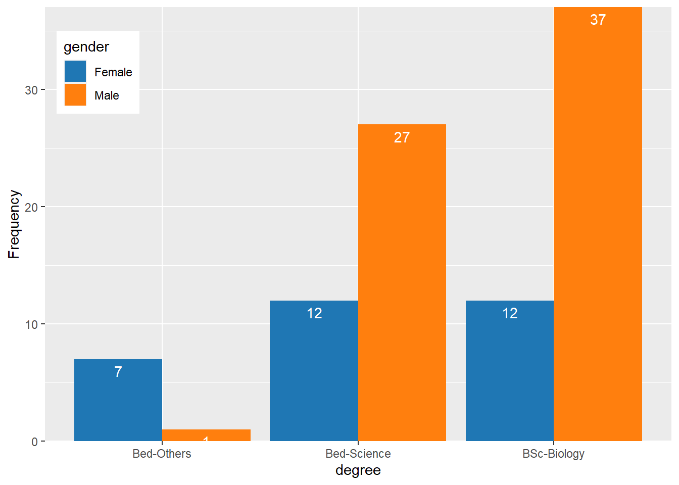
qns %>%
  select(degree = 9, gender = Gender) %>%
  ggplot(aes(x = degree))+
  geom_bar(fill = "maroon")+
  facet_wrap(~gender)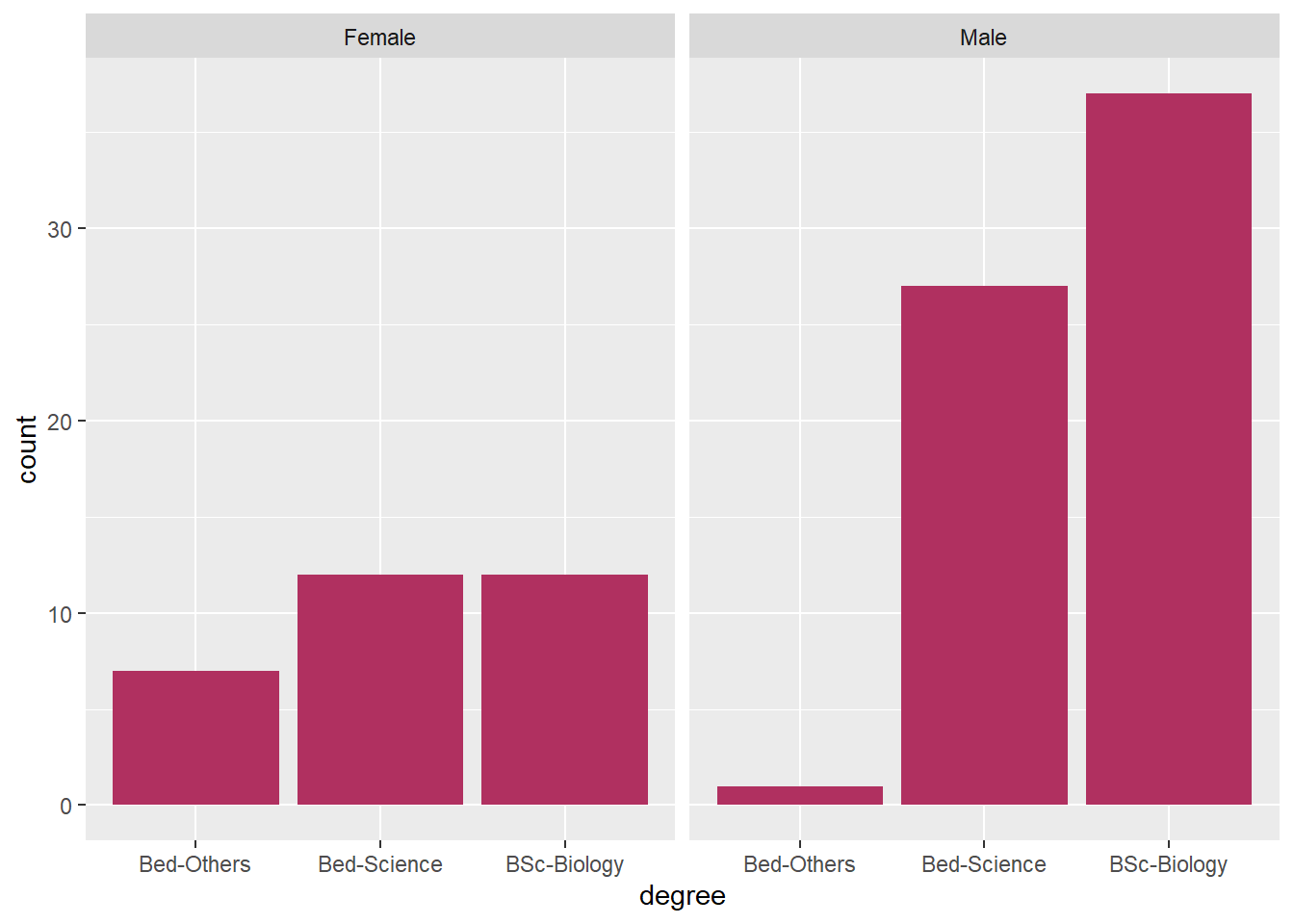
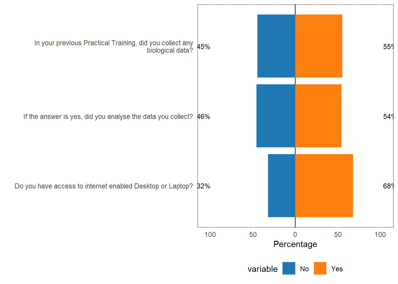
multiple response
likert.re = qns %>%
  mutate(across(is.character, as.factor)) %>%
  as.data.frame() %>%
  dplyr::select(12,21,22) %>%
  likert()

  likert.re
Item
1 Do you have access to internet enabled Desktop or Laptop?
2 In your previous Practical Training, did you collect any biological data?
3 If the answer is yes, did you analyse the data you collect?
No Yes
1 32.29167 67.70833
2 44.79167 55.20833
3 45.83333 54.16667likert.re %>%
plot(ordered = F, wrap= 60)+
ggsci::scale_fill_d3()