Wind Data in R with rWind package

The Global Forecasting System (GFS) atmospheric model is a dataset from the National Oceanic and Atmospheric Administration (NOAA) and National Centers for Environmental Prediction (NCEP). In this database, wind is stored as velocity vector components (U: eastward_wind and V: northward_wind) at 10 m above the Earth’s surface. The resolution of the data is 0.5 degrees, approximately 50 km. Wind velocities have been registered six times per day (00:00 – 03:00 – 06:00 – 09:00 – 12:00 – 15:00 – 18:00 – 21:00 (UTC)), since 6th May 2011 and is updated daily.

Fernández-López and Schliep (2019) developed rWind package that allows to query and access raw plain text file with gridded data, with the date and time of the data, the location (longitude and latitude coordinates) the wind vectors (U and V components) and wind speed and direction. These data can either be exported in a .csv file or stored internally as an ‘rWind data frame’ in R. In this post, we are going to learn how to download wind data and plot them. First we load the packages we are going to use in this session.

require(tidyverse)
require(rWind)
require(sf)
require(patchwork)
require(ggspatial)

Our interest is to have weekly wind data from June 01, 2021 to December 31, 2021. To capture the period, we create a date sequence vector object with an interval of seven days using lubridate package (Grolemund and Wickham 2011).

dt = seq(lubridate::dmy(010621),
         lubridate::dmy(311221), by = "7 day")

Then we define our area of interest that fall within geographical extent of longitude 35–55 and latitude -25–10.

Once we know the geographical extent and created the date object of the time period we want to download the data, we can parse those argument into the wind.dl_2 function, which allows us to download time-series wind data from the Global Forecast System (GFS) of the USA’s National Weather Services. Wind data are taken from NOAA/NCEP Global Forecast System (GFS) Atmospheric Model collection and has spatial resolution of 0.5 degrees (approximately 50 km) at the equator, and wind is calculated at 10 m from the Earth surface.

wind.series = wind.dl_2(time = dt, lon1 = 30, lon2 = 60, lat1 = -25,lat2 = 10)

We also extract basemap of African simple feature from spData package and crop to the area of interest with st_crop function from sf package (Pebesma 2018).

wio = spData::world %>% 
  filter(continent == "Africa") %>% 
  st_crop(xmin = 32.5,xmax = 53,ymin = -26,ymax = 6)

We then color code for visualization

mycolor2 = c("#040ED8", "#2050FF", "#4196FF", "#6DC1FF", "#86D9FF", "#9CEEFF", "#AFF5FF", "#CEFFFF", "#FFFE47", "#FFEB00", "#FFC400", "#FF9000", "#FF4800", "#FF0000", "#D50000", "#9E0000")
mycolor = c("#7f007f", "#0000ff",  "#007fff", "#00ffff", "#00bf00", "#7fdf00",
"#ffff00", "#ff7f00", "#ff3f00", "#ff0000", "#bf0000")
odv_color = c("#feb483", "#d31f2a", "#ffc000", "#27ab19", "#0db5e6", "#7139fe", "#d16cfa") %>% rev()
pal = wesanderson::wes_palette("Zissou1", 21, type = "continuous")
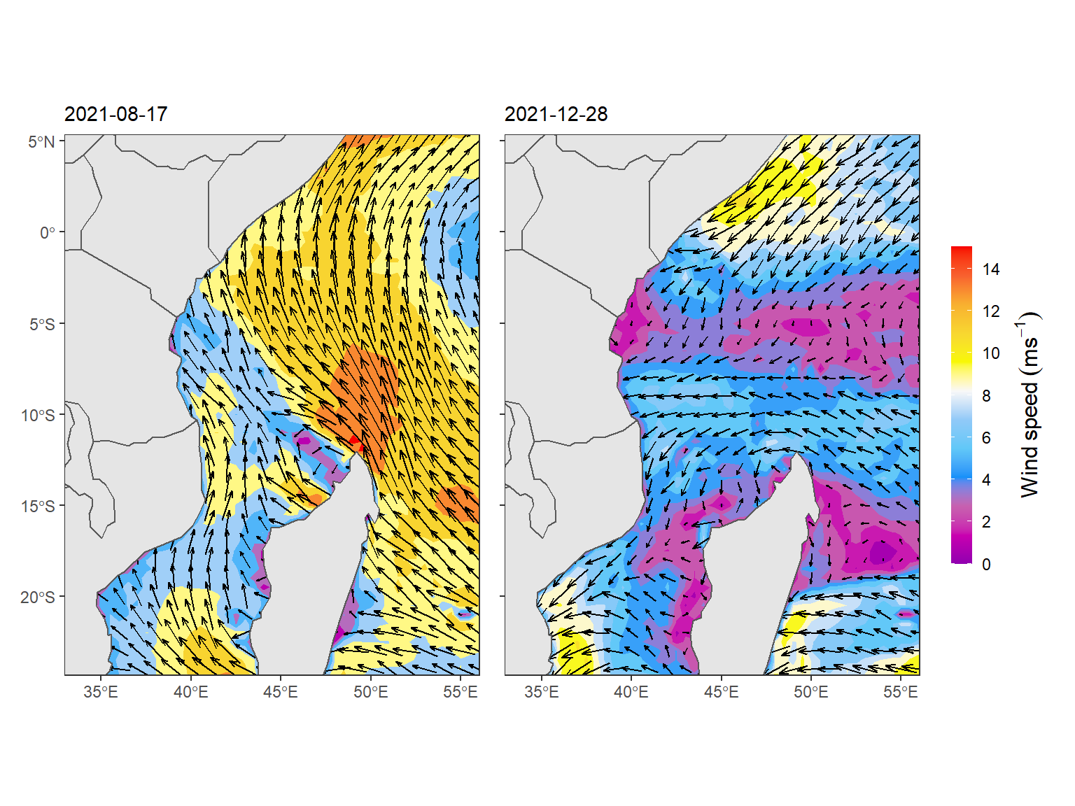
mycolor3 = c("#9000B0", "#C900B0", "#C760AF",                    "#1190F9", "#60C8F8", "#90C9F8", "#F8F8F8", "#F8F800",  "#F8D730", "#f8b030", "#f8602f", "#f80000")

We then combine the power of grammar of graphic (ggplot2) (Wickham 2016) and sister package metR (Campitelli 2019) to plot wind speed as filled contour and overlay velocity components zonal and meridional as vector layer as the code below shows.

aug = wind.series[[12]] %>% as_tibble() %>% 
  ggplot(aes(x = lon, y = lat))+
  metR::geom_contour_fill(aes(z = speed))+
  # metR::geom_contour2(aes(z = speed), breaks = seq(4,20,4))+
  metR::geom_vector(aes(dx = ugrd10m, dy = vgrd10m), skip = 1, show.legend = FALSE, 
                    preserve.dir = TRUE, arrow.type = "open", arrow.angle = 20)+
  scale_fill_gradientn(colours = mycolor3, 
                       limits = c(0,15), 
                       breaks = scales::breaks_pretty(n = 10),
                       guide = guide_colorbar(title = "Speed(m/s)", 
                                              barwidth = unit(.4,"cm"), 
                                              barheight = unit(6,"cm")))+
  ggspatial::layer_spatial(data = wio)+
  coord_sf(xlim = c(34,55), ylim = c(-23,4))+
  metR::scale_mag(max = 15)+
  theme_bw()+
  theme(axis.title = element_blank(), legend.position = "none")+
  labs(subtitle = wind.series[[12]]$time %>% unique())


dec = wind.series[[31]] %>% as_tibble() %>% 
  ggplot(aes(x = lon, y = lat))+
  metR::geom_contour_fill(aes(z = speed))+
  # metR::geom_contour2(aes(z = speed), breaks = seq(4,20,4))+
  metR::geom_vector(aes(dx = ugrd10m, dy = vgrd10m), skip = 1, show.legend = FALSE, 
                    preserve.dir = TRUE, arrow.type = "open", arrow.angle = 20)+
  scale_fill_gradientn(colours = mycolor3, 
                       limits = c(0,15), 
                       breaks = scales::breaks_pretty(n = 10),
                       guide = guide_colorbar(title = expression(Wind~speed~(ms^{-1})), 
                                              title.position = "right",
                                              title.theme = element_text(angle = 90),
                                              title.hjust = .5,
                                              barwidth = unit(.4,"cm"), 
                                              barheight = unit(6,"cm")))+
  ggspatial::layer_spatial(data = wio)+
  coord_sf(xlim = c(34,55), ylim = c(-23,4))+
  metR::scale_mag(max = 15)+
  theme_bw()+
  theme(axis.title = element_blank(), axis.text.y = element_blank())+
  labs(subtitle = wind.series[[31]]$time %>% unique())

aug + dec