
Local Spatial Autocorrelation
Introduction
In this post, we explore the analysis of local spatial autocorrelation statistics, focusing on the concept and its most common implementation in the form of the Local Moran statistic. We explore how it can be utilized to discover hot spots and cold spots in the data, as well as spatial outliers. To illustrate these techniques, we will use the catch data from Deep Sea fishing authority.
Moran’s I
Moran’s I statistic is arguably the most commonly used indicator of global spatial autocorrelation. It was initially suggested by Moran (1948), and popularized through the classic work on spatial autocorrelation by Cliff and Ord (1973). In essence, it is a cross-product statistic between a variable and its spatial lag, with the variable expressed in deviations from its mean. observations.
LISA Principle
As we have seen Moran I are designed to reject the null hypothesis of spatial randomness in favor of an alternative of clustering. Such clustering is a characteristic of the complete spatial pattern and does not provide an indication of the location of the clusters. The concept of a local indicator of spatial association, or LISA was suggested in Anselin (1995) to remedies this situation.
A LISA is seen as having two important characteristics. First, it provides a statistic for each location with an assessment of significance. Second, it establishes a proportional relationship between the sum of the local statistics and a corresponding global statistic.
Most global spatial autocorrelation statistics can be expressed as a double sum over the i and j indices, such as \((\sum_i \sum_j g_{ij})\). The local form of such a statistic would then be, for each observation (location) \(\(i\)\), the sum of the relevant expression over the \((j)\) index, \((\sum_j g_{ij})\).
More precisely, a spatial autocorrelation statistic consists of a combination of a measure of attribute similarity between a pair of observations, \((f(x_i,x_j))\), with an indicator for geographical or locational similarity, in the form of spatial weights, \((w_{ij})\). For a global statistic, this takes on the form \((\sum_i \sum_j w_{ij}f(x_i,x_j))\). A generic form for a local indicator of spatial association is then: \([\sum_j w_{ij}f(x_i,x_j).]\) As there are many statistics for global spatial autocorrelation, there will be many corresponding LISA. In this Chapter, we focus on the local counterpart of Moran’s I.
Local Moran
As discussed by Ord and Getis (1995), the local Moran and Getis–Ord statistics both are useful as methods to detect clusters and share a fundamental underlying mathematical relationship. However, in the way the two statistics are used, the two methods consider clusters to be somewhat distinct concepts. The Getis–Ord Gi statistic (in its Zi form) focuses on whether or not the area around \(i\) tends to be larger or smaller than a typical local sum.
The local Moran statistic, in contrast, focuses on clusters around sites where the local covariation is more positive than is expected, given the global structure of covariation between nearby sites. Further, both statistics preserve the proportionality and significance properties proposed by Anselin (1995) and thus are both local indicators of spatial association. As further noted by Anselin (1995), the two types of statistics also share a fundamental similarity in terms of their inferential value under permutation inference (p. 100).
So, we will not discuss the permutation inference for the Gi statistic here and note that an identical conditional randomization strategy is used as in the local Moran’s I dataset. Thus, despite the fact that the Moran-style statistics examine the local covariation and the Getis–Ord statistics examine the local sum, both are useful in characterizing the local structure of how observations cluster with respect to the rest of the map.
Implementation
Xun Li and Luc Anselin (2021) developed a rgeoda package, R Library for Spatial Data Analysis. The package has several tools for spatial analysis. Among the many tools is a local_geary function, which is used to compute the Getis-Ord’s local G* statistics. You can install the package as
install.packages("rgeoda")Once installed, you can load the package function in your session using require function
require(rgeoda)We aldo add some other packages that are useful in the session as follows;
require(tidyverse)
require(sf)
require(magrittr)
require(patchwork)
ps = read_csv("../eez_stock assessment/processed_purse_seine.csv")Then we create a simple feature from a dataframe
tuna.cpue.sf = ps %>%
  select(category_name, longitude, latitude, wt_mt)%>%
  distinct(longitude, latitude, category_name, .keep_all = TRUE)%>%
  wior::outlier_remove(wt_mt) %>%
  st_as_sf(coords = c("longitude", "latitude"), crs = 4326)
Load basemaps that will be used to plots maps
africa.countries= st_read("d:/semba/pfz/shapefile/africa.shp", quiet = TRUE)%>%
  st_simplify(dTolerance = 0.005, preserveTopology = TRUE)

tz.sf = africa.countries %>% st_crop(xmin = 38, ymin = -14, xmax = 43, ymax = -3)
Filter the point object and discard category_name variable from the dataset
yf.sf = tuna.cpue.sf %>%
  # filter(category_name == "Yellowfin") %>%
  select(-category_name)
Then compute the local morans. As shown in the chunk below, the local spatial statistic G is calculated for each point based on the spatial weights object used. The value returned is a Z-value, and may be used as a diagnostic tool.
the first step is to create a weighted
yf.getis = yf.sf %>%
  rgeoda::queen_weights() %>%
  local_gstar(df = yf.sf)

labels = yf.getis %>% lisa_labels()
colors = yf.getis %>% lisa_colors()
We then plot with ggplot
raw.data = yf.sf %>%
  ggplot() +
  geom_sf(aes(color = wt_mt)) +
  ggspatial::layer_spatial(data = tz.sf) +
  coord_sf(xlim = c(38.4,43.1), ylim = c(-10.5,-4.8))+
  theme_bw()+
  scale_color_gradientn(colors = oce::oce.colors9A(120), name = "Catch (MT)")

hot.cold = yf.sf %>%
  mutate(clusters = yf.getis %>% lisa_clusters()) %>%
  ggplot() +
  geom_sf(aes(color = clusters %>% as_factor())) +
  ggspatial::layer_spatial(data = tz.sf) +
  coord_sf(xlim = c(38.4,43.1), ylim = c(-10.5,-4.8))+
  theme_bw()+
  scale_color_manual(values = c("grey80", "red", "blue"), labels = labels, name = "Getis Ord")

raw.data + hot.cold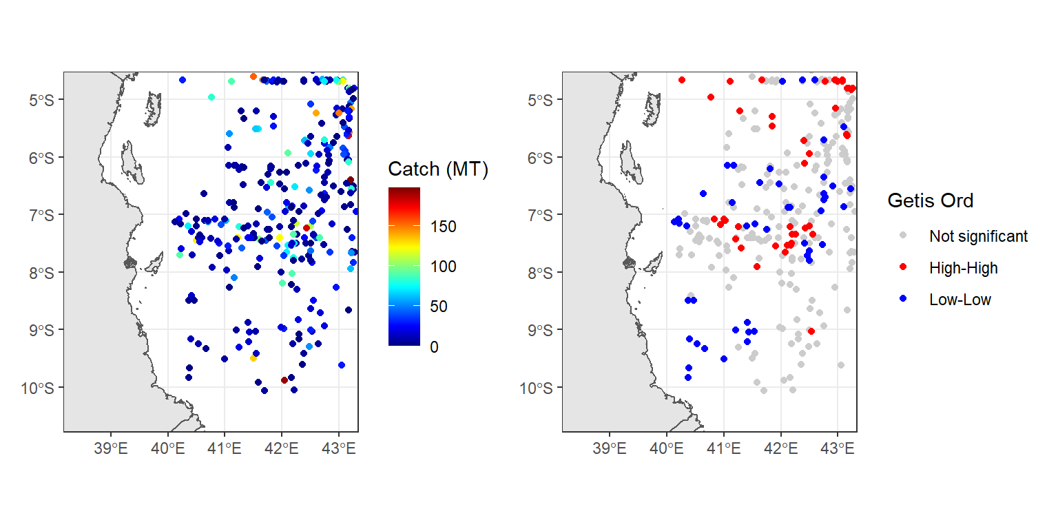
Figure 1: Hotspot and coldspot of catch rates in the EEZ waters of Tanzania
The interpretation of the local Getis–Ord statistic is shown in Figure 1, the capture weight of tuna in the Exclusive Economic Zone of Tanzania are shown on the left, with the Getis–Ord Gi statistics on right for three distinct bandwidth values. High positive values indicate the possibility of a local cluster of high values of the variable being analysed, very low relative values a similar cluster of low values.
Conclusion
The Getis–Ord Gi statistic is a distinct perspective on the question of geographical clustering from other measures, like the Local Geary’s ci or Local Moran’s Ii statistics. The Getis–Ord Gi statistic measures whether the area around site \(i\) tends to be larger (or smaller) than areas that are not near site \(i\). In general, when the area around \(i\) is significantly larger (or smaller) than would be observed at random, then site \(i\) is considered to be the core of a “hotspot” (or coldspot). Unlike Moran’s I, the Gi statistic is only concerned with identifying clusters and does not identify spatial outliers, observations that are strongly dissimilar to their surroundings.
Bonus
## smooth catch rate
tuna.kernel = tuna.cpue.sf %>%
  st_transform(crs = 32737) %>%
  wior::point_tb() %>%
  select(-category_name) %>%
  rename(x = lon, y = lat) %>%
  btb::kernelSmoothing(sEPSG = "32737", iCellSize = 20000, iBandwidth = 30000, vQuantiles = .5) %>%
  st_transform(4326)
number of clusters: 1
Median smoothing progress (parallel clusters): 100% - minimum remaining time: 0m 0s
Elapsed time median smoothing: 0m 0s density.catch = tuna.kernel %>%
ggplot()+
geom_sf(aes(fill = wt_mt_05))+
scale_fill_gradientn(colours = oce::oce.colors9A(120), trans = scales::boxcox_trans(p = .2))+
ggspatial::layer_spatial(data = tz.sf) +
coord_sf(xlim = c(38.4,43.1), ylim = c(-10.5,-4.8))+
theme_bw()
## compute local moran
moran = tuna.kernel %>%
select(wt_mt_05) %>%
rgeoda::queen_weights() %>%
local_gstar(df = tuna.kernel)
labels = moran %>% lisa_labels()
colors = moran %>% lisa_colors()
hot.cold.catch = tuna.kernel %>%
mutate(clusters = lisa_clusters(moran)) %>%
filter(!clusters >=4) %>%
ggplot() +
geom_sf(aes(fill = clusters %>% as.factor()))+
scale_fill_manual(values = moran %>% lisa_colors(), label = moran %>% lisa_labels(), name = "Clusters")+
ggspatial::layer_spatial(data = tz.sf) +
coord_sf(xlim = c(38.4,43.1), ylim = c(-10.5,-4.8))+
theme_bw()
density.catch + hot.cold.catch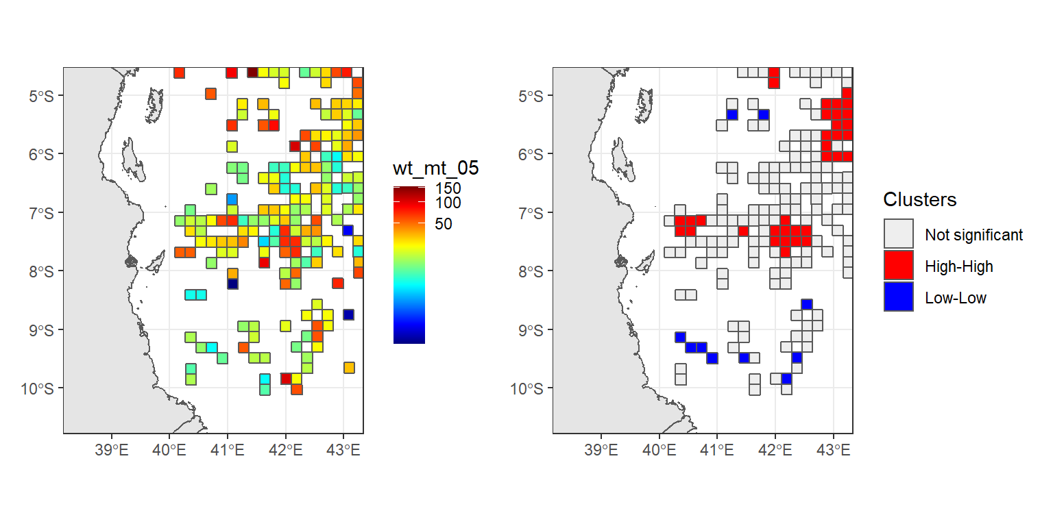
Figure 2: Raw catch (left) and Hotspot and coldspot of catch rates (right) in the EEZ waters of Tanzania
