Google trends in R

Google Trends is a well-known, free tool provided by Google that allows you to analyse the popularity of top search queries on its Google search engine. In market exploration work, we often use Google Trends to get a very quick view of what behaviours, language, and general things are trending in a market.

Philippe Massicotte’s developed a gtrendsR package for running Google Trends queries in R. It’s simple, you don’t need to set up API keys or anything, and it’s fairly intuitive. Let’s have a go at this with a simple and recent example.

gtrendsR is available on CRAN, so just make sure it’s installed (install.packages(“gtrendsR”)) and load it. Let’s load tidyverse as well, which we’ll need for the basic data cleaning and plotting:

require(gtrendsR)
require(tidyverse)

The next step then is to assign our search terms to a character variable called search_terms, and then use the package’s main function gtrends().

Let’s set the geo argument to Hong Kong only, and limit the search period to 12 months prior to today. We’ll assign the output to a variable - and let’s call it output_results.

trends = gtrends(keyword = c("John Magufuli"),
                       geo = c("UG", "TZ", "KE"),
                       time = "2014-01-01 2022-01-30")

class(trends)

[1] "gtrends" "list"   

Let’s have a look at interest_over_time, which is primarily what we’re interested in. You can access the data frame with the $ operator, and check out the data structure:

trends.tb = trends$interest_over_time %>% 
  mutate(hits = as.integer(hits))

trends.tb %>% 
  dplyr::slice_sample(n = 10)

         date hits       keyword geo                  time gprop category
1  2014-06-01    0 John Magufuli  KE 2014-01-01 2022-01-30   web        0
2  2014-01-01    1 John Magufuli  TZ 2014-01-01 2022-01-30   web        0
3  2019-06-01   NA John Magufuli  UG 2014-01-01 2022-01-30   web        0
4  2019-04-01    7 John Magufuli  TZ 2014-01-01 2022-01-30   web        0
5  2018-06-01    3 John Magufuli  TZ 2014-01-01 2022-01-30   web        0
6  2015-10-01   NA John Magufuli  UG 2014-01-01 2022-01-30   web        0
7  2020-03-01   NA John Magufuli  KE 2014-01-01 2022-01-30   web        0
8  2016-12-01   NA John Magufuli  KE 2014-01-01 2022-01-30   web        0
9  2017-01-01   16 John Magufuli  TZ 2014-01-01 2022-01-30   web        0
10 2015-06-01    5 John Magufuli  TZ 2014-01-01 2022-01-30   web        0

trends.tb%>% 
  ggplot(aes(x = date, y = hits, color = geo))+
  geom_path()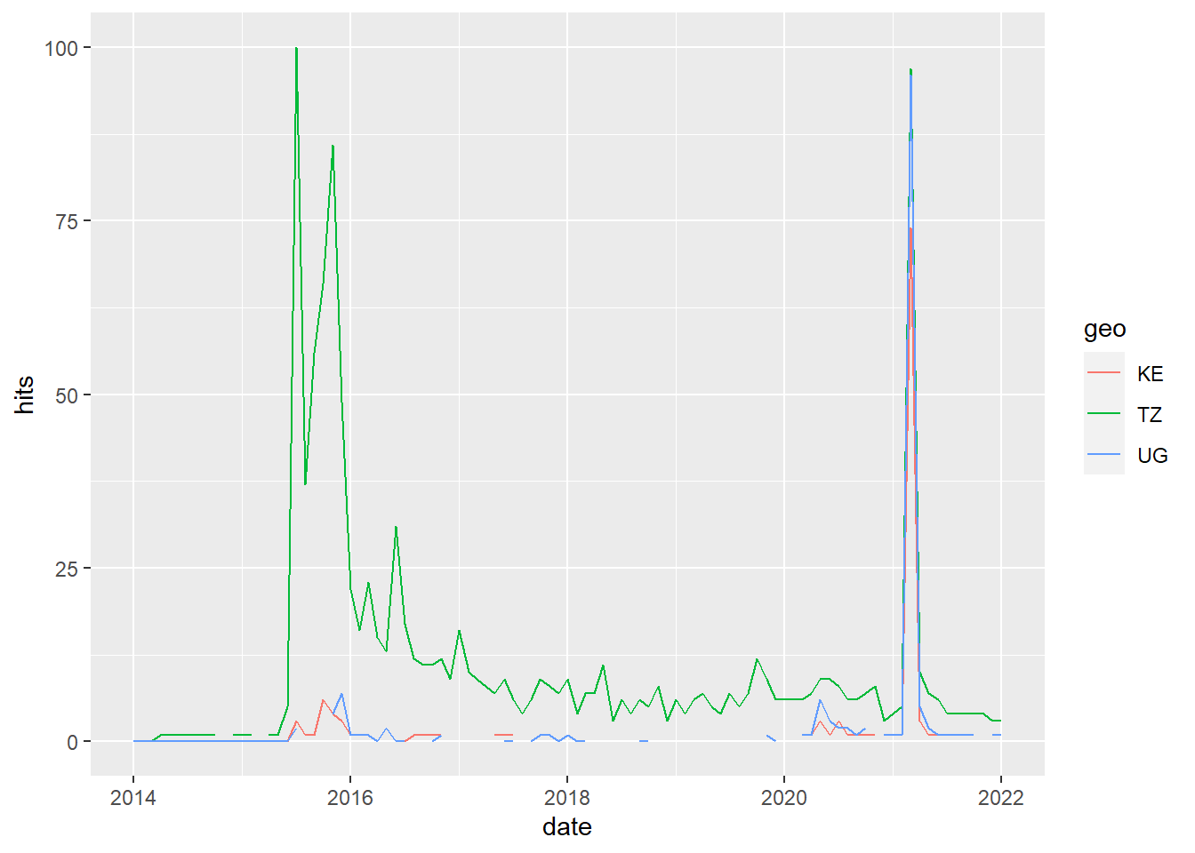

YOu will notice that the hits are below 100, Why? According to Google FAQ documentation:

Google Trends normalizes search data to make comparisons between terms easier. Search results are normalized to the time and location of a query by the following process. Each data point is divided by the total searches of the geography and time range it represents to compare relative popularity. Otherwise, places with the most search volume would always be ranked highest.The resulting numbers are then scaled on a range of 0 to 100 based on a topic’s proportion to all searches on all topics.